A pinch of OR in Biostatistics

The first thing in common between Operational Research (OR) and Biostatistics, is that both terms are often misunderstood. OR, or the Science of Better, as it is commonly known, has lots to do with optimization but there is much more to it…Some might be surprised to read that many of the tools of this discipline can be -and are actually- applied to problems in Biostatistics.

It all starts with Florence Nightingale volunteering as a nurse in the Crimean war in 1853…Her pioneering use of statistics for evidence-based medicine, and her operational research vision to reform nursing, led to a decline in the many preventable deaths that occurred throughout the nineteenth century in English military and civilian hospitals.

Since then, integrated approaches are commonplace: disease forecasting models, neural networks in Epidemiology, discrete-event simulation in clinical trials,…

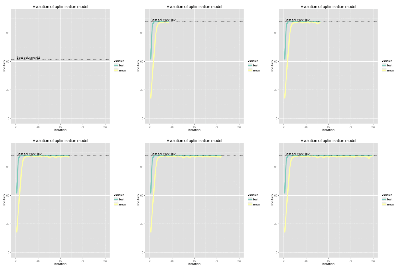
Figure: Genetic algorithm representation using R. Find here the code for the original dynamical plot by FishyOperations.

There is also an increasing interest in computational biology in OR. Examples of application of these techniques vary from linear programming based flux balance analysis models for cell metabolism studies, to sparse network estimation in the area of Genetics.

In R, there are many packages with which to apply these techniques, from genalg for Genetic algorithms (used to recreate figure above) or games on Games theory, to more specific packages in Bioconductor like CellNOptR, survcomp or OLIN. Also, a general Task View on Optimization can be found here.

Finally, a quick mention to the YoungOR 18 Conference that will be held in Exeter (UK), 9-11 April 2013. It will be covering topics of common interest for biostatisticians with streams on Health, Sustainability, etc. Plenty of inspiration for future posts!

Have you ever used any of these techniques?Any particular tips that you want to share?Tell us about it!

Biostatistics in a Health Services Environment

Aurora Baluja is MD in the Department of Anesthesiology, Intensive Care and Pain Management of the Hospital Clinico Universitario of Santiago de Compostela, and PhD candidate at the Forensic Medicine Unit of the University of Santiago de Compostela (Spain).

As a medical doctor involved in patient management, -in operating room and in the ICU-, every day I witness the huge load of data that has to be processed, interpreted, and stored. In this situation, Biostatistics and Bioinformatics support becomes greatly important to analyse trends and patterns, that ultimately lead to improve patient care.

I do research about risk profiles of mortality in the ICU, and given the amount of data obtained, the task of reporting my results and ensure reproducibility became very time-consuming.

In this post I intend to comment on the main tools that helped me so much to overcome those obstacles:

R: for me, the possibility of learning a statistical computing language to write and recycle scripts, was definitely the way. R is a powerful, open source programming language and software environment, that allows a full variety of analyses and… beautiful graphs.
RStudio: to find a good IDE for R code was also important. Fortunately, Altea recommended me this easy-to-use, visual piece of cake, with integrated options to report code and results… Thanks!
R Markdown is a quick, easy method to write scripts and to report clean code and results, with some formatting options, in an HTML page. It is implemented in R-studio by the package “knitr”. Just one click away, you can generate a complete, dynamic report with text and graphics.
LaTeX: the main reason for me to use LaTeX is not writing documents with beautiful symbols and equations, but to somehow link my R console to a document editor, in order to generate tables and reports, just like I do with R Markdown. For this, I need to use R-studio again, and 4 more ingredients:

A LaTeX distribution: I have installed TeX Live for Linux, and MiKTeX for MS Windows. A variety of templates, included often in distributions, make the first approach quite easy. Beyond the use of Sweave (see below), I became so fond of LaTeX that now it is my favourite text editor for documents, posters and slides!
R Sweave is the link between R-scripts and LaTeX, making possible to write an entire LaTeX document with dynamic results from R commands embedded in it.
Texreg: maybe the reason why I’ll never quit using LaTeX. Its magic begins after you have run several models of your data, and you are trying to see and compare *all* of them at a glance. It generates latex-formatted tables with your models, ready to paste into a LaTeX document. As a tip, I often use them preserving their \{tabular} environments and customising \{table} options to fit my document style.
Xtable: another R package, that allows to print nice tables in LaTeX format.

I encourage those who haven’t used any of these tools, to give them a try… surely they will help you!

Measuring Disease Trends through Social Media

Nichole Knupp is a freelance blogger and marketing professional who writes guest posts and website content for a variety of different blogs and niches that interest her.

People in the field of Medicine, those in Master´s in Public Health programs (see examples here and here) or in other disciplines such as Biostatistics (see previous post on the topic) might wonder how social media can play a valid role in their career. While social media has taken the world by storm, it has mostly been thought of as a tool for sharing personal information, marketing, or keeping up on the latest gossip. However, after this past flu season, those in the medical and scientific fields are finding a whole new way to use information that is trending. Here are just a few of the things that social media is doing to benefit our health and sciences community.

Measuring Disease Trends
One of the terms being used for those watching and tracking the spread of illnesses through social media is “social media analytics” (see for instance, social network analysis). Quite simply, it is tracking outbreaks of various viruses through mining social media. This past season, people were following the spread of influenza through a flu hash tag (#flu). Viruses such as H1N1 and the Swine Flu were able to be monitored on Twitter. Further, they found when information was extracted efficiently, it was accurate and there was even a possibility of forecasting further trends. The most pertinent information though, was what was happening in the present. Different agencies were able to find what area was the hardest hit and who was at risk.

Public Interest and Concerns
The health and sciences community also found social media to be a great platform in finding out how interested the public was in disease outbreaks and trends. It was also a way to gather concerns so various agencies could address them. Social media is utilized by people as a way to have their voices heard through an outlet that is part of their daily lives. While some people are unwilling to sit down and answer a survey, important information can be gathered by what is mentioned on daily Twitter streams.

Disease Outbreaks and Travel
Since social media is a tool that is being used worldwide, it has also been helpful in tracking outbreaks abroad. US citizens, and others traveling, can easily be informed through public social media announcements. Currently there are conversations happening on how best to use the information gathered on social media, and what role it will play in informing the public and addressing questions and concerns. (A very interesting article on the topic can be found here).

Social Media Sources
While Twitter has been the main source used for tracking trends, Instagram, Facebook, and Google Trends also play a part. Some places to look if you’re interested in seeing how it all works is checking out the HealthMap stream on Twitter (@healthmap), do a Google Trends “flu” search, or try a flu hash tag search (#flu) on Twitter.

It’s not hard to imagine the possibilities and many other things we will be able to track in the future, but one thing is already certain— there is a use for social media if you work in the medical sciences, Public Health, Biostatistics,…

Do we need Spatial Statistics? When?

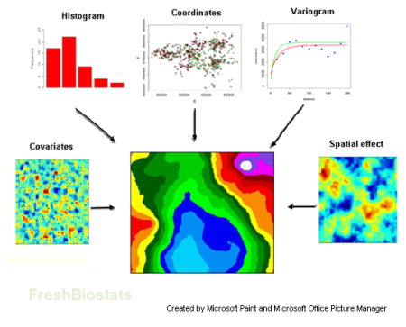
Spatial Statistics, What is it? and Why use it?

The approach taken in this post is to offer an introduction of basic and main concepts of spatial data analysis as well as the importance of its utilization in some areas like epidemiology or ecology among others. But, before to introduce a definition of spatial statistics and some concepts about this field, I consider relevant to mention some situations in which our data need to be seen as ‘spatial data’.

It is possible that people associate spatial statistics with analysis that contain numerous maps. However, it goes beyond creating these, in fact spatial data analysis is subject to internal structure of the observed data. We therefore have to be careful with the questions not directly answered by looking at the data.

We could make a long list of areas where we can apply spatial statistics: epidemiology, agriculture, ecology, environmental science, geology, meteorology, oceanography,… even econometrics. In all of these we could ask questions like the following to recognize if our data have a spatial structure:

Does the distribution of cases of a disease form a pattern in space?Could we relate health outcomes to geographic risk factors?
Do they influence environmental and geographical factors in the distribution and variability in the occurrence of fishery species?

But, how can we explain what is spatial statistics? I am sure that we could find infinite definitions of spatial analysis or spatial statistics. We can say that spatial statistics is responsible for analyzing the variability of random phenomena that are linked with their geographic locations. It is used to model the dependence of the georeferenced observations (these can be point observations or areal data).

Depending on the type of data and the purpose of the spatial analysis itself, we classify spatial data sets into one of three basic types: geostatistical data, lattice data (or areal data) and point pattern data. The main dissimilarity between these resides in the set of observations. Let us look at this briefly with some examples:

Geostatistics: the geostatistical data are represented by a random vector $Y(s)$ , where the locations $s \in D$ varies continuously over a fixed observational region ( $D \subset \Re^{r}$ ). These data are characterized by spatial dependence between the locations, and the main objective in application of geostatistics is to do predictions in unobserved locations from study region. kriging is the best known technique for prediction in geostatistical data. Some examples of this data are: occurrence of species in a region, annual acid rain deposition in a town, etc.

Lattice data: the fixed subset ( $D \subset \Re^{r}$ ) of observations are located in a continuous region (it can have a regular or irregular shape). It is partitioned into a finite number of geographical areas with well-defined boundaries. A characterization of this type of spatial data is that neighbouring areas are usually more similar than distant ones. An example can be the observed locations from agricultural field trials (here the plots are a regular lattice).

Point pattern data: this is the last type of spatial data where $D \subset \Re^{r}$ is itself random. The own locations determined phenomena that occurred randomly in one place, thus generating spatial patterns. One example of point pattern data is the locations of a certain species of tree in a forest (here only the locations are thought of as random).

The above explanation have only been a briefly description of three main types of spatial data. There are two basic methodologies to carry out spatial analysis: through classical statistics or by Bayesian approach (using mainly hierarchical Bayesian methods). The latter will be dealt with in more detail in future posts, given their importance as they can be applied in many situations, like spatial statistics (you can see the book ‘Hierarchical Modeling and Analysis for Spatial Data by Banerjee et al.’ for more information about this).

The complex structure of the longitudinal models

Two weeks ago, we started to talk in this blog about longitudinal data with the post by Urko Agirre. This type of data involves complex structure models called longitudinal models.

Longitudinal studies have two important characteristics:

They are multivariate because for each studied individual many temporal measurements from the response variable (and covariates) are collected.
They are multilevel as the variables measured are nested within the subjects under study, therefore resulting in layers.

These characteristics allow us to make inference about the general trend of the population as well as about the specific differences between subjects that can evolve in another way regarding the overall average behavior.

At the beginning of the 20th century this type of data started to be modelled. Different proposals appeared such as ANOVA models (Fisher, 1918), MANOVA models (generalised from ANOVA models to multivariate) or growth curves (Grizzle and Allen, 1969). All these proposals showed improvements in some aspects. However, they left some others unresolved. On the one hand, ANOVA models are univariate and our data are multivariate. On the other hand, MANOVA models are multivariate but assume independence between intra-subject observations (observations from the same individual are not independent in general). Finally, the last option, growth curves, contemplate intra-subject observations dependence but are too restrictive on the design matrix.

It was not until the early 80s when a proposal that included all the aspects of these complex data appeared. Laird and Ware proposed the application of linear mixed models (LMM) in the paper “Random-Effects Models for Longitudinal Data“.

The basic structure of these LMM of each patient $i$ is:

$y_i = X'_i\beta + Z'_ib_{i} + W_i(t_i) + \epsilon_i$

where

$y_i=(y_{i1},...y_{in_i})$ is the vector of measurements of the response variable, made to ith a total of $m$ subjects in times $t_i=(t_{i1},...t_{in_i})$ . $n_i$ is the number of repeated measured of the ith patient.
$X'_i\beta$ represents the deterministic model, being $X'_i$ the submatrix design covariates associated with the ith individual, and $\beta$ its associated parameter vector.
$Z'_ib_i$ are random effects responsible for capturing the variability between individuals.
$W_i(t_i)$ includes intra individual variability, ie the variability between observations of the same subject.
Finally, $\epsilon_i$ reflects the variability that is not due to any kind of systematic error that we can determine.