Featured

P-splines for longitudinal data

Ipek

Ipek Guler is an intern at Biostatech, Advice, Training and Innovation in Biostatistics, S.L. She has a MSc in Statistical Techniques from the University of Santiago de Compostela (Spain) and a BSc in Statistics from Gazi University (Turkey).

Contact Ipek

In previous posts about longitudinal data by Urko Agirre and Hèctor Perpiñán, mentions have already been made to the Mixed Models methodology .

Usually in medical and biological studies, the designed experiments include repeated measures which are used to investigate changes during a period of time repeatedly for each subject in the study. Multiple measurements are obtained for each individual at different times. These type of longitudinal data can be analyzed with a mixed effects model (Pinheiro and Bates, 2000) which allows modeling and analysis of between and within individual variation. An example of such data can be growth curves measured over time.

In many practical situations, using traditional parametric regression techniques is not appropriate to model such curves. Misleading conclusions may be reached if the time effect is incorrectly specified.

Durban et al, (2005) presented flexible mixed models for fitting subject specific curves and factor by curve interactions for longitudinal data in which the individual and interaction curves are modeled as penalized-splines (P-splines) and model’s estimation is based on the mixed model representation of P-splines (Currie and Durban, 2002).

This representation is quite interesting because it allows us to use the methodology and the several software available for mixed models (e.g., nlme and lme4 packages in R), and it also comes equipped with an automatic smoothing parameter choice that corresponds to maximum likelihood (ML) and/or restricted maximum likelihood (REML) estimation of variance components. With this representation, the smoothing parameter becomes the ratio between the variance of residuals and the variance of the random effects.

First of all, let`s define a linear mixed model for a longitudinal data.

As a matrix notation;

y=X\beta+Zu+\varepsilon

  • y is the vector of the observed responses ,

\left(\begin{array}{cc}y_{1}\\\vdots\\ y_{n}\end{array}\right)=\left(\begin{array}{cc}y_{11}\\y_{12}\\\vdots\\ y_{1n_{1}}\\ y_{2_{1}}\\\cdot\\\cdot\\\cdot\end{array}\right)

  • \beta is the fixed effects parameters vector,
  •  \varepsilon=\left(\begin{array}{cc}\varepsilon_{1}\\\varepsilon_{2}\\\vdots\\ \varepsilon_{N}\end{array}\right)  is the residual vector,
  •  u=\left[\begin{array}{cc}u_{1}\\u_{2}\\\vdots\\ u_{N}\end{array}\right] denotes unknown individual effects.
  • Z=\left[\begin{array}{ccc}Z_{1}&\ldots&0\\\vdots&\ldots&\vdots\\ 0&\ldots&Z_{N}\end{array}\right]  a known designed matrix linking u to y,
  • X=\left[\begin{array}{cc}X_{1}\\X_{2}\\\vdots\\ X_{N}\end{array}\right]

  u_{i}, i=1,\ldots,N assumed to be N(0,G), independently of each other and of the \varepsilon_{i}.\varepsilon_{i} is distributed as N(0,R_{i}) where R_{i} and G_{i}  are positive definitive covariance matrices.

Consider a flexible regression model,

y_{i}=f(x_{i})+\varepsilon_{i}

\varepsilon_{i}\sim N(0,\sigma^2)

Where y_{i} is the response variable of the observations i=1 ,\ldots, N and f(\cdot) is the smooth function of covariate x. We represent this function with a linear combination of d known basis function B_{j}.

And we reformulate it as;

y=B\theta+\varepsilon

\varepsilon\sim N(0,\sigma^2I)

Depending on the basis that is used for the P-splines, X and Z have the following forms;

  • Truncated polynomials

X=\left[1,x,\ldots,x^p\right]
Z=\left[(x_{i}-\kappa _{k})^p_+\right]
1 \leqslant i \leqslant n
1\leqslant k \leqslant \kappa

  • B-splines

X=[1:x]

Z=BU\Sigma^{-1/2}

Where U  is the matrix that contains the eigenvectors of the singular value decomposition of the penalty matrix  P=D\prime D and \Sigma   is a diagonal matrix containing the eigenvalues with q null eigen values (Lee, 2010).

Therefore the model becomes;

y=X\beta+Zu+\varepsilon

u\sim N(0,\sigma^2_{u}I_{c-2})

and \varepsilon\sim N(0,\sigma^2I)

Where c is the number of columns of basis B, and the smoothing parameter becomes; =\frac{\sigma^2}{\sigma^2_{u}} (Durban et al, 2005).

With this mixed model representation of P-splines, we can obtain more flexible mixed models which allows us to have a simple implementation of otherwise complicated models. In future posts, we can talk more about these flexible models with individual curves and factor by curve interactions also described in Durban et al (2005).

Featured

SPSS, SAS or R…which one to choose?

Performing statistical analyses by hand in the era of new technologies would seem crazy.  Nowadays, there are three main statistical programs for doing statistics: IBM SPSS, SAS  and R, as it can be read in a more extensive post of this site. Sometimes, biostatisticians need to use more than one package to carry out their analyses.  This means that users of these programs have to move from one to another environment, from front-end to back-end, using different wizard and graphical interfaces, wasting in most occasions an important amount of time. Because of that, in this post I would like to address the differences between the aforementioned programs, pointing out the advantages and the most suitable usage of each software from my personal point of view.

For a good choice of a statistical program, one should take into account several issues such as the following:

1. Habit: It refers to how the biostatistician has gotten used to one particular statistical program and does not need to learn something new.

2. Distrust of freeware: it refers to the license type of the package.

3. Availability of statistical procedures:  are the most used statistical methods included in the package?

4. Management of huge data sets: how big data sets are handled.

Focusing on the first point, it is remarkable that programming with these three packages is quite easy. All of them provide a choice to write the syntax code and run it whenever you want. This also can be applied to anyone who might have to send you the code, including managers or colleagues. Besides, IBM SPSS and R offer a friendly interface allowing the alternative of not learning the syntax procedure. These could be the main reasons for which people continue doing data analysis for a long period with the same statistical program, making a better researcher life!

Another important issue is whether the distribution is freeware or not. When starting to work as a biostatistician, one soon notices the high cost of statistical software licence fees. As you might know, IBM SPSS and SAS are commercial distributions and  R is freeware. Although IBM SPSS and SAS are quite expensive, one should think about the benefits that both programs offer in the long term. For example, some researchers do not trust R, and think its use does not ensure getting the correct results. In those cases, trust comes at a price. Regadless of what they think, R has grown rapidly in the past few years, offering competition to other softwares.

The availability of the most used statistical procedures is another important point to be taken into account.  All of them have integrated in their environments the most popular statistical methods (regression analysis, correspondence analysis, etc..) but sometimes, there is a need for implementing more sophisticated procedures.  As IBM SPSS and SAS are paid-for distributions, they do not let the user to program it, they have fixed instructions. On the contrary, R could be understood as a combined and customized software of multiple small packages to solve the problems. Whenever you have a problem, it is most likely that you will find a solution for it in the packages repository.

Finally, as for the management of huge data sets, it is noteworthy that SAS is the winner. SAS has a robust platform for handling big data sets and it does not  need the whole computer memory for the analysis. In this sense, R still has a long way to go even though the performance of R in this area has recently been exponentially increased. I would also say that IBM SPSS does not have enough support.

To sum up, I would like to give a couple of advices. From the point of view of my experience, I would recommend to use IBM SPSS for medical researchers who start doing statistics: it is quite easy and intuitive and there is no need to learn the syntax. But not for a long period of time: learning basic R coding is not difficult and will be sufficient for the requirements of this type of researchers. It is only a small effort but really worthy! Nonetheless, for advanced researchers and biostatisticians, a combination between SAS and R would be perfect – that is what I do!, I would say I am RSAS user… -. Now, you have the choice: IBM SPSS, SAS or…R?

Featured

…a scientific crowd

While researching on scale-free networks, I found this book, which happens to include the very interesting article The structure of scientific collaboration networks and that will serve me as a follow-up to my previous post on social networks here.

Collaborative efforts lie in the foundations of the daily work of biostatisticians. As such, the analysis of these relationships –lack of interaction in some cases- appears to me as fascinating.

The article itself deals with the wider community of scientists, and connections are understood in terms of papers´ co-authorships. The study seems to prove the high presence of small world networks in the scientific community. However short the distance between pairs of scientists I wonder, though, how hard it is to cover that path, i.e., are we really willing to interact with colleagues outside our environment? Is the fear to step out of our comfort zone stopping us from pursuing new biostatistical challenges? Interestingly, one of Newman´s findings amongst researchers in the areas of physics, computer science, biology and medicine is that “two scientists are much more likely to have collaborated if they have a third common collaborator than are two scientists chosen at random from the community.”

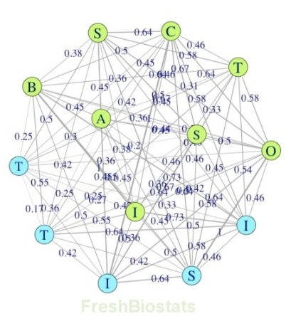
Interaction patterns analyzed through social networks diagrams like the one shown in Fig 1., can give us a hint on these patterns of collaboration, but can also be a means towards understanding the spread of information and research in the area (ironically, in a similar fashion to the spread of diseases as explained here). sociogram_biostatistics

Fig.1. Biostatistics sociogram (illustration purposes only; R code adapted from here and here)

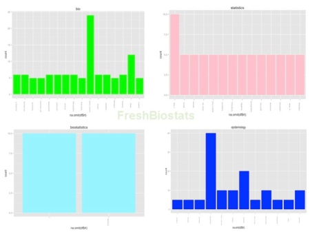
In my previous post on the topic, I focused on the great Linkedin inmaps. I will be looking this time at Twitter and an example of the huge amount of information and the great opportunities for analysis that the platform provides. R with its package twitteR makes it even easier… After adapting the code from a really useful post (see here), I obtained data relating to twitter users and the number of times they used certain hashtags (see plots in Fig. 2).

twitter_counts

Fig.2. Frequency counts for #bio (top left), #statistics (top right), #biostatistics (bottom left), and #epidemiology (bottom right). Twitter account accessed on the 17th of May 2013.

Although not an exhaustive analysis, it is interesting to notice the lower figures for #biostatistics (turquoise) and #statistics (pink), compared to #bio (green) and #epidemiology (blue) for example (please notice the different scales in the y axis for the four plots). It makes me wonder if the activity in the field is not our strongest point and whether it would be a fantastic way to promote our profession. I am certainly convinced of the great benefits a higher presence in the media would have, particularly in making it more attractive for the younger generations.

That was just a little peek of even more exciting analysis to come up in future posts, meanwhile see you on the media!

Do you make any use of the social networks in your work? Any interesting findings? Can´t wait to hear them all!

Featured

A computational tool for applying bayesian methods in simple situations

Luis Carlos SilvaLuis Carlos Silva Ayçaguer. Senior researcher of the Escuela Nacional de Salud Pública from La Habana, Cuba; member of the development team of Epidat. Degree in Mathematics from Universidad de La Habana (1976), PhD from Universidad Carolina (Praga, 1982), Doctor of Science from Universidad de Ciencias Médicas (La Habana, 1999), Titular Academic from República de Cuba.
 
Email: lcsilva@infomed.sld.cu

Web: http://lcsilva.sbhac.net

Soly SantiagoSoly Santiago Pérez. Technical statistician at Dirección Xeral de Innovación e Xestión da Saúde Pública (General Directorate of Public Health, Spain) from 1996 to present; member of the development team of Epidat. Degree in Mathematics from Universidad de Santiago de Compostela (Spain, 1994). Specialist in Statistics and Operational Research.

Email: soly.santiago.perez@sergas.es

In this post, we present a user friendly tool for applying bayesian methods in simple situations. This tool is part of a free distribution software package, Epidat, that is being developed by the Dirección Xeral de Innovación e Xestión da Saúde Pública (Xunta de Galicia, Spain) since the early 90’s. The general purpose of Epidat is to provide an alternative to other statistical packages for performing analysis of data; more specifically, it brings together a broad range of statistical and epidemiological techniques under a common interface. At present, the fourth version of Epidat, developed in Java, is freely available from the web page: http://dxsp.sergas.es; to download the program, registration is required.

As stated above, one of the methods or “modules” included in Epidat 4 is Bayesian analysis, a tool for the application of bayesian techniques to basic problems, like the estimation and comparison of means and proportions. The module provides a simple approach to Bayesian methods, not based on hierarchical models that go beyond the scope of Epidat.

The module of Bayesian analysis is organized into several sub-modules with the following scheme:

  • Bayes’ theorem
  • Odds ratio
  • Proportion
    • One population
      • Estimation of a proportion
      • Assessment of hypotheses
    • Two populations
      • Estimation of effects
      • Assessment of hypotheses
  • Mean
    • One population
      • Estimation of a mean
      • Assessment of hypotheses
    • Two populations
      • Estimation of a difference
      • Assessment of hypotheses
  • Bayesian approach to conventional tests

The first option of the module can be used to apply Bayes’ theorem. The following three options (Odds ratio, Proportion and Mean) are designed to solve basic inferential problems under Bayesian logic: estimation of odds ratios, proportions and means, as well as differences or ratios of these two last parameters. The punctual estimation is accompanied by the corresponding credibility interval. The techniques available in these options also include methods related to hypothesis testing. Finally, the last sub-module allows the evaluation of conventional tests from a Bayesian perspective.

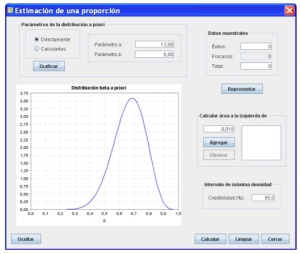
Estimation of a proportion

Some specific options of Bayesian analysis require the use of simulation techniques. Nevertheless, the user does not need to understand the simulation process to use the program and interpret the results correctly. In addition, the module has a user-friendly interface that allows the user to plot the a priori distribution and choose the values of its parameters (see figure above). The output of Bayesian analysis includes both numerical and graphical results, and the graphics can be edited and modified by the user. In addition, the contents of the output window can be saved as a file in several formats: *.epi, *.pdf, *.odf, or *.rtf.

Finally, like all modules of Epidat, Bayesian analysis has a useful help feature which can be accessed on the help menu in pdf format. This facility has been developed with a didactic and critical approach, including statistical basics of the methods, bibliographic references, and examples of the different options.

R2wd package: another tool to create reports

The last post published in FreshBiostats, by Hèctor Perpiñán, was about reports combining the use of R and Latex. In it, he explained how to transport tables and figures from the R output to Latex.

Well then, this week I shall continue talking about another tool to write reports when we do the statistical analysis with R. It allows us to reduce the time spent to draft the reports and be more accurate by minimising human copying errors. I am going to focus my attention on “R2wd” package to write MS-Word documents from R.

Although most statisticians are used to work daily with Latex which results in high quality appearance, in most cases our clients have never heard about it and prefer to work with MS-Word documents, which are easier to handle.

The R2wd package needs either the statconnDCOM server (via the rcom package) or the RDCOMClient to communicate with MS-Word via the COM interface. Once this interface is installed (on Windows OS), we can create a document using all functions available in this package: wdGet, wdTitle, wdSection, wdType, wdSetFont, wdTable (the object must be a data frame or an array), wdPlot, wdApplyTheme, etc.

Not only do these functions allow us to introduce tables or figures from R output, but can also be used to inject text elements into Word report, themes and templates, different type of text (normal, italic, Verbatim,…), etc.

The following code shows a little example on how to use this package:

</pre>
### An easy example to use "R2wd" package ###

library("R2wd") #of course, you must install it before!
#require("rcom")

wdGet() #To open a new Word document

#It is possible that we get an error message with wdGet() function.
#In this case we will need to install:
#installstatconnDCOM()

wdTitle("We introduce here our file title")
wdSection("First section begins here")

wdBody("Inserts text in 'Body' style at the current cursor point in Word.")
wdWrite("The function wdBody is similar to 'wdWrite'",paragraph=TRUE)
wdType("Now we use an italic type and a centering text",italic=TRUE,alignment="center")
wdNormal("To return a Normal type")
wdWrite("We can also insert footnotes")
wdInsertFootnote("insert a footnote") #you can insert footnotes in the
#word document at the cursor position.

wdSection("Now we include another section")
wdSubsection("A toy example")

wdBody("Insert tables of results")

age <- c(23,12,45,34,18,41)
gender <- c(1,1,0,1,0,0)
height <- c(172, 150,169,180,188,160)
data <- data.frame(age,gender,height)

wdTable(data,autoformat=2)#three possibilities to autoformat parameter
wdItemize()
wdWrite("insert a text in the bullet",paragraph=TRUE)
wdItemize(Template=3)
wdWrite("we finish the description",paragraph=TRUE)
wdBody("To finish this easy example we include a plot in our Word document")

wdPlot(data$age,data$height,col="red",pch=20,height = 10, width =10, pointsize = 25)

wdSave()
wdQuit() #To close the session

As you have seen, besides being able to format our report as we want (although it may seem cumbersome to do from R), R2wd is really useful because with an only function – wdTable() – and one “click” I can copy a large table in my report with no mistakes.

You will find more functions here. Dare to try it! You will save plenty of time!