In the last post I provided a simple introduction about spatial data and how to begin to manipulate them. Now, I would like to continue showing you some simple examples about what we could do with these data and the R tools we apply when working with them. Throughout this post I introduce you some links where R tools to process and learn about spatial data are available.
We continue using the same Spanish shapefile downloaded here.
Remember you need to load the library ‘maptools’ to read the shapefile.
#load the autonomous communities shapefile:
library(maptools)
map1 <- readShapeSpatial('ESP_adm1.shp')
To plot this map you only need the ‘plot()’ function, but here I want to introduce a slightly different method of creating plots in R: the ‘ggplot2’ package. There is so much information about this package that you can find. For example, this web site http://ggplot2.org/ provides you with some useful books (R Graphics Cookbook (book website) and ggplot2: Elegant Graphics for Data Analysis (book website) where you can learn about this package. Also you can find presentations with examples and the corresponding R code.
‘ggplot()’ function requires some previous steps to prepare the spatial data: it needs to transform our SpatialPolygonsDataFrame into a standard data frame. For this, ‘rgeos’ package must be installed.
library(ggplot2)
library(rgeos)
map1.ggplot = fortify(map1, region="ID_1")
#Now map1.ggplot is a data.frame object
‘fortity()’ function converts a generic R object into a data frame that needs the ggplot function. The ‘region’ argument determines that the variable for each geographical area is identified and this should be common to both the map and the data.
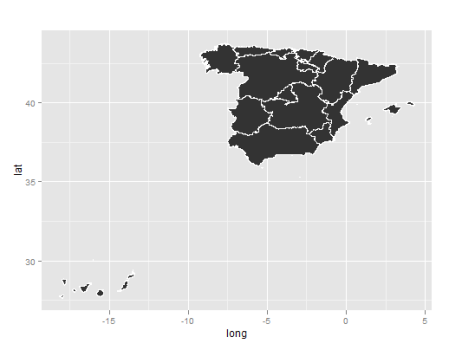
A simple map is obtained with the following call to ggplot():
g <- ggplot(data = map1.ggplot, aes(x = long, y = lat, group = group)) +
     geom_polygon() +
     geom_path(color="white") + coord_equal()
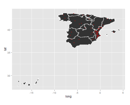
If we want to add over the map a set of points:
#add points
locations <- read.csv('locations.csv',header=T)
g + geom_point(aes(long, lat,group=NULL), colour = "red", size = 0.3,  data = locations)
#locations should be a data frame object
If you want to test the code, you can generate points using the ‘locator()’ function and then create with them a data frame.
Finally, I would like to introduce the ‘over()’ function in the sp package to process spatial overlays and extractions. Let us suppose that we have a set of points over the region, and we only need the locations of one community. To use that function, we need to work with spatial objects.
# To create a SpatialPoints
coordinates(locations) <- c("long","lat")
# And to define the CRS:
proj4string(locations) <- CRS("+proj=utm +zone=30 +ellps=WGS84")</i></pre>

# Select the region of ‘Comunidad Valenciana’
map_Val <- map1[which(map1@data$NAME_1=="Comunidad Valenciana"),]
# CRS:
proj4string(map_Val) <- CRS("+proj=utm +zone=30 +ellps=WGS84")

pos<-which(!is.na(over(locations, geometry(map_Val))))
locnew <- locations[pos,]
pos stores the indices of the locations that are within the map_Val (discard the points that are out). After this point, you should follow the same steps to plot map_Val and the locnew points with the ggplot function.
I hope that beginners in spatial data find this information helpful!


