Shiny, a simple and powerful tool to create web-based applications using R

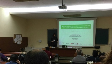
Isaac Subirana holds a MSc in Science and Statistical Techniques from the Universitat Politècnica de Catalunya (UPC) in 2005. Additionally, he was awarded his PhD in Statistics from the Universitat de Barcelona (UB) in 2014. Since 2007 he has been teaching statistics and mathematics at the faculty of Biology (UB) and Statistics (UPC) as associate professor. Since 2004 he has been working at REGICOR group (IMIM-Parc de Salut Mar) assessing statistical analyses in cardiovascular and genetic epidemiological studies. He has given several workshops of Shiny, at UPC Summer School, Servei d’Estadística Aplicada de la Universitat Autònoma de Bellaterra (SEA-UAB), at Basque Country University (EHU) and at the Institut Català d’Oncologia (ICO).

 

In the last decade, R has become one of the most used software both for statistical and data-analysis in general. On the one hand, R offers a great flexibility and power to perform any kind of analyses and computations. On the other, R has a very steep learning curve for beginners while other software such as SPSS are much more intuitive and easier to learn. By far, these point-and-click alternatives are the most commonly used by analysts who do not have the knowledge to manage R commands with confidence. It would appear that many physicians and researchers from other applied areas belong to this group of people who feel much more comfortable using this sort of software than writing commands.

The problem arises when a complex statistical analysis not implemented in SPSS-like software is required for a paper publication, e. g. spline models to assess dose-response effects. In such cases a researcher unfamiliar with R may enlist the help of a statistician to do the analysis. This prevents the researcher from performing data exploration or repeating the analyses by selecting groups of individuals, for instance, to create or confirm hypotheses. To overcome this situation, the statistician could provide the researcher with an R syntax indicating where to modify the code. However, this is not an optimal solution because the researcher would have to deal with an unfamiliar language and run a code that may return unintelligible error messages.

Some efforts have been done to bring R to less proficient users by building Graphical User Interfaces (GUIs). One of the most well-known examples is Rcmdr which is an R package to perform general statistical analyses. In addition, there are numerous Rcmdr plug-ins packages performing more specific analyses such as survival analyses, etc. Both, Rcmdr and their plug-ins, are built using tcltk tools (tcltk2 R package). By using tcltk2 it is possible to create and customize windows, buttons, lists, etc., but its syntax is not very intuitive, at least for R users. Other existing alternatives consist on using web program languages (HTML, Javascript and PHP) which also allow to plug-in R commands. The problem is that most R users are not familiar with HTML, Javascript or PHP, and building even a simple application may be too demanding.

In 2012, a new R package called Shiny was submitted to R CRAN repository (see Pilar’s post on the topic here). It was created and is maintained by Joe Cheng and collaborators from the RStudio team. Unlike tcltk2, Shiny is much more intuitive and simple. Shiny wraps HTML and Javascript using exclusively R instructions to create web based GUIs which can be opened from any internet explorer (such as Chrome, Firefox, etc.). Therefore, Shiny takes all the power of HTML, Javascript and R without having to know anything of the first two. From a usability point of view, the main advantage of creating GUIs applications with Shiny is that they can be called from any device (see this page for more details). On the Shiny website there are a lot of examples and a very extensive list of tutorials and article. I would strongly recommend that you visit it before starting to create an application with Shiny.

Since Shiny was first presented in useR 2013 conference in Albacete its popularity has grown exponentially. More and more R packages incorporates its GUI built with Shiny; compareGroups to build descriptive tables, MAVIS for meta-analyses, Factoshiny which is a Shiny-web GUI of FactoMineR package for factor analyses, or GOexpress for genomic data analyses are some examples. Even a section in R-bloggers has been created exclusively for Shiny topics (see this website). And specific Shiny conferences are taking place (see this website).

By default, Shiny applications may look too minimalistic, and sometimes, their functionality could be seen as limited. To improve Shiny applications aspect and functionality, there are some R packages available on CRAN. Of special interest are shinythemes which incorporates a list of CSS templates, shinyBS  to build modals or shinyjs  which wraps Javascript code.

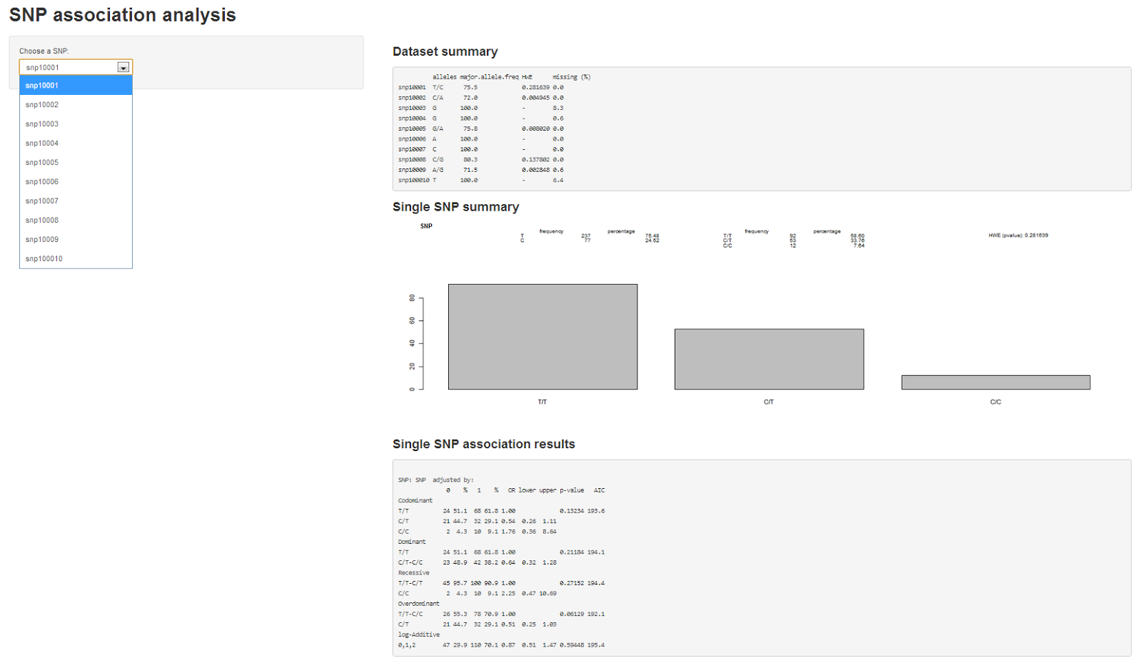
I started using Shiny to create a GUI for compareGroups, an R package to build descriptive tables for which I am the maintainer. We found the necessity to open the compareGroups package to SPSS-like software users not familiar with R. To do so, it was necessary to create an intuitive GUI which could be used remotely without having to install R, upload your data in different formats (specially, SPSS and Excel), select variables, and other options with drop-down lists and buttons. You can take a look at the compareGroups project website for further information. Aside from developing the compareGroups GUI, during these last three years I have also been designing other Shiny applications, ranging from performing models (website) to teaching statistics in the university (website).

In conclusion, Shiny is a great tool to be used by R-users who are not familiar with HTML, Javascript or PHP to create very flexible and powerful web-based applications.

If you know how to do something in R, you can make other non-R users do it by themselves too!

 

Recent developments in joint modelling of longitudinal and survival data: dynamic predictions

by Guest Blogger Ipek Guler

Following previous posts on longitudinal analysis with time-to-event data, I would like to resume recent developments in joint modelling approaches which have gained a remarkable attention in the literature over recent years.

Joint modelling approaches to the analysis of longitudinal and time-to-event data are used to handle the association between longitudinal biomarkers and time-to-event data on follow-up studies. Previous research on joint modelling has mostly concentrated on single longitudinal and single time-to-event data. This methodological research has a wide range of biomedical applications and statistical software package facilities. There are also several extensions to joint modelling approaches such as the use of flexible longitudinal profiles using multiplicative random effects (Ding and Wang, 2008), alternatives to the common parametric assumptions for the random effects distribution (Brown and Ibrahim, 2003), and handling multiple failure times (Elashoff et al, 2008). For nice overviews on the topic, read Tsiatis and Davidian (2004) and Gould et al (2015). Beside these developments currently the interest lies on multiple longitudinal and time-to-event data (you can find a nice overview of multivariate joint modelling in Hickey et al. (2016)).

In this post, I will focus on an interesting feature of joint modelling approaches linked to an increasing interest in medical research towards personalized medicine.  Decision making based on the characteristics of individual patients optimizes the medical care and it is hoped that patients who are informed about their individual health risk will adjust their lifestyles according to their illness. That information often includes survival probabilities and predictions for future biomarker levels which joint models provide.

Specifically, subject-specific predictions for longitudinal and survival outcomes can be derived from the joint model (Rizopoulos 2011 & 2012). Those predictions have a dynamic nature coming from the effect of repeated measures taken in time t to the survival up to time t. This allows updating the prediction when we have new information recorded for the patient.

Rizopoulos (2011) uses a Bayesian formulation of the problem and Monte Carlo estimates of the conditional predictions with the MCMC sample from the posterior distribution of the parameters for the original data. The R package JMbayes calculates these subject-specific predictions for the survival and longitudinal outcomes using  the functions survfitJM() and predict(), respectively. As an illustration, the following functions can be utilized to derive predictions for a specific patient from the Mayo Clinic Primary Biliary Cirrhosis Data (PBC) dataset using a joint model.

library("JMbayes")
library("lattice")
data("pbc2")
data("pbc2.id")

pbc2$status2 <- as.numeric(pbc2$status != "alive")
pbc2.id$status2 <- as.numeric(pbc2.id$status != "alive")

## First we fit the joint model for repeated serum bilirumin
## measurements and the risk of death (Fleming, T., Harrington, D., 1991)

lmeFit.pbc <-
  lme(log(serBilir) ~ ns(year, 2),
      data = pbc2,
      random = ~ ns(year, 2) | id)
coxFit.pbc <-
  coxph(Surv(years, status2) ~ drug * age, data = pbc2.id, x = TRUE)
jointFit.pbc <-
  jointModelBayes(lmeFit.pbc, coxFit.pbc, timeVar = "year", n.iter = 30000)

## We extract the data of the patient 2 in a separate data frame
## for a specific dynamic predictions:

ND <- pbc2[pbc2$id == 2,]
write.table(ND,"pbc2.csv",sep=";",dec=",",row.names=FALSE)

sfit.pbc <- survfitJM(jointFit.pbc, newdata = ND)

#The plot()
#method for objects created by survfitJM() produces the figure
#of estimated conditional survival probabilities for Patient 2

plot(
  sfit.pbc,
  estimator = "mean",
  include.y = TRUE,
  conf.int = TRUE,
  fill.area = TRUE,
  col.area = "lightgrey"
)

## In a similar manner, predictions for the longitudinal outcome
## are calculated by the predict() function
## For example, predictions of future log serum bilirubin
## levels for Patient 2 are produced with the following code: 

Ps.pbc <- predict(
  jointFit.pbc,
  newdata = ND,
  type = "Subject",
  interval = "confidence",
  return = TRUE
)

## Plotting the dynamic predictions of the longitudinal measurements

last.time <- with(Ps.pbc, year[!is.na(low)][1])
xyplot(
  pred  + low + upp ~ year,
  data = Ps.pbc,
  type = "l",
  lty = c(1, 2, 2),
  col = c(2, 1, 1),
  abline = list(v = last.time, lty = 3),
  xlab = "Time (years)",
  ylab = "Predicted log(serum bilirubin)"
)

Furthermore, Rizopoulos (2014) presents a very useful tool for clinicians to present the results of joint models via a web interface using RStudio Shiny (see a previous post by Pilar on this here).  This is available in the demo folder of the package JMbayes and can be invoked with a call to the runDynPred() function. Several options are provided in the web interface such as predictions in case you have more than one model in the workspace based on different joint models, obtaining estimates at specific horizon times and extracting a dataset with the estimated conditional survival probabilities. Load your workspace and your new data (as described in the data tab just after you load your workspace), choose your model and select one of the interesting plots and representative tools. A detailed description of the options in this app is provided in the “Help” tab within the app.

Just try the code above and see!

References

• Brown, E. R., Ibrahim, J. G. and Degruttola, V. (2005). A flexible B-spline model for multiple longitudinal biomarkers and survival. Biometrics 61, 6473.
• Ding, J. and Wang, J.-L. (2008). Modeling longitudinal data with nonparametric multiplicative random effects jointly with survival data. Biometrics 64, 546 – 556.
• Gould AL, Boye ME, Crowther MJ, Ibrahim JG, Quartey G, Micallef S, Bois FY.  (2015) Joint modeling of survival and longitudinal non-survival data: current methods and issues. Report of the DIA Bayesian joint modeling working group. Stat Med., 34, 2181–2195.
• Hickey, G.L., Philipson, P., Jorgensen, A. et al. (2016) Joint modelling of time-to-event and multivariate longitudinal outcomes: recent developments and issues. BMC Medical Research Methodology. 16: 117.
• Rizopoulos D (2011). Dynamic Predictions and Prospective Accuracy in Joint Models for Longitudinal and Time-to-Event Data.  Biometrics, 67, 819–829.
• Rizopoulos D (2012). Joint Models for Longitudinal and Time-to-Event Data, with Applications in R. Chapman & Hall/CRC, Boca Raton.
• Tsiatis, A. and Davidian, M. (2004). Joint modeling of longitudinal and time-to-event data: An overview. Statistica Sinica 14, 809 – 834.

p-values explained

David Blanco (UPC) recently prepared this video following the ASA statement  and we wanted to share it with you. We particularly love the very useful examples (who would not want those work colleagues?!) and the BNE Shiny application.

We also highly recommend this RSS video on the development and impact of the statement, including some very interesting discussions.

We hope you find it useful, please do share your thoughts!

Reflections from “Dance your PhD”

by Guest Blogger Ipek Guler

In 2015, Ipek Guler submitted a video to the competition “Dance your  PhD” sponsored by Science/AAAS, organisation which each year encourages researchers to represent their work in the form of a dance.

You can check out her video below:

and read her reflections on the experience below:

How did you hear about the competition and why did you decide to enter?

I heard about the competition on John Bohannon’s TED talk where he gives a brilliant example of how to turn a presentation into a dance with a professional contemporary dance company. He talks about how the lasers cool down matter. Amazing! I think I had already decided to do it right at the beginning of the talk. As i do perform contemporary dancing as a semi-professional dancer, the idea was perfect for me.

Where  did you find the inspiration to translate biostatistical concepts into dance?

There are some inspiring sentences on the Dance Your PhD website: “So, what’s your Ph.D. research about?” You take a deep breath and launch into the explanation. People’s eyes begin to glaze over… At times like these, don’t you wish you could just turn to the nearest computer and show people an online video of your Ph.D. thesis interpreted in dance form?”

So this was my starting point. I was very excited to be able to explain my research to my friends, parents, relatives finally. The other good point was that I used it to introduce different concepts, feelings into my dance performances; this is what you are able to do in contemporary dancing that other forms of academic dissemination do not allow.

How  long did it  take you to finish  the video?

For a long time I had already been trying to summarise my PhD research to other people who have no idea about statistics. The process of translating it into dance helped me a lot for my future presentations and in my thesis.

The choreography took a few months to create in my mind. The next step was the rehearsal  with my dance group. It was the fastest and easiest process which took a few days because we used to create, dance and improvise together for years. Finally we shot the video in one day and had  lots of fun (we also added some of these moments at the end of the video. :))

Would you recommend it to other PhDs in Biostatistics?

I definitely recommend it to other researchers in Biostatistics who have just finished their PhD or are still PhD students. First of all you will able to resume your principal aim, the most important points of your PhD research, then you’ll have a great product to show when you are not able to explain to other people who have no idea what you are doing. Especially in biostatistics, people sometimes don’t understand what you’re really doing, so you have a brilliant option. Believe me, it works!

You can watch other Dance your PhD videos on mathematics here and  here, and some biomedical ones too here and here.

Review of the 3rd Biostatnet General Meeting “Facing challenges in biostatistical research with international projection”

(Photo from Biostatech website)

Following on from successful meetings back in January 2011 and 2013,  on the 20-21 January 2017 Biostatnet members gathered again in Santiago to celebrate the network’s successes and discuss future challenges. These are our highlights:

Invited speakers

The plenary talk, “Why I Do Clinical Trials: Design and Statistical Analysis Plans for the INVESTED Trial”, introduced by Guadalupe Gómez Melis, was given by Prof. KyungMann Kim, from the Biostatistics and Medical Informatics department at the University of Wisconsin. Prof. Kim discussed challenges faced when conducting clinical trials to ensure follow-up of patients, and the technological and statistical conflicts in the endeavour to make large-scale clinical trials cost-efficient.

Prof. KyungMann Kim’s presenting his work

The invited talk by Miguel Ángel Martínez Beneito from FISABIO showcased solutions to issues with excess zeros modelling in disease mapping in a very enjoyable talk that generated a fascinating discussion.

Inmaculada Arostegui introducing Miguel Ángel Beneito’s talk

Roundtables

We really enjoyed the two great roundtables that were held at the meeting.

Young Researchers Roundtable

Firstly, we were delighted to be given the opportunity to organise a roundtable of young researchers at the event, and although we did not have much time, we managed to squeeze in four main topics of discussion including; Biostatnet research visits, reproducibility in research, professional visibility and diversity with a focus on women in Biostatistics (very fittingly just before the celebrations of the 1st International Day of Women and Girls in Science!). The topics proved to be of great interest and raised a lively discussion. Regarding visibility, issues such as how to properly manage a professional online profile and what the potential risks of too much exposure are, were raised in the discussion. Also mentioned was the fact that, while there is no doubt that accessing data and code for replicability and reproducibility purposes is highly important, researchers might lose sight of the conclusions due to a major focus on having full access to these resources.

Some other interesting issues were prompted that we could not expand on (we would have needed more time…!) so we would like to continue here…Feel free to send us your comments either here or via social media! or to answer this brief survey (post here). We are currently preparing a paper summarising the topics covered in the roundtable and we will let you know when it is ready!

Participants in the roundtable from right to left: Danilo Alvares (with contributions from Elena Lázaro), Miguel Branco, Marta Bofill, Irantzu Barrio and María José López.

BIO Scientific Associations Roundtable

Secondly, a very exciting and lively session gathering researchers with different backgrounds, all members of a variety of BIO associations and networks, gave us their impressions about what it means to work within a multidisciplinary team. In a very constructive and lively atmosphere, promoted by the moderator Erik Cobo (UPC), Juan de Dios Luna (Biostatnet), Vitor Rodrigues (CIMAGO), Mabel Loza (REDEFAR) and Marta Pavía (SCReN) discussed the pitfalls in communication between statisticians and researchers. We all really enjoyed this session, and took home some valuable messages to improve the interactions between (bio)statisticians, clinicians and applied researchers.

Workshops

In addition to a satellite course on “CGAMLSS using R” (post to come on this topic!), we had the opportunity to attend two workshops on the last morning of the meeting.

Juan Manuel Rodriguez and Licesio Rodríguez delivered the Experimental Designs workshop. In a very funny and lively way (and using paper helicopters!!!!), they reviewed key concepts of Experimental Designs. This helpful workshop gave us a great opportunity to dust off our design toolkit.

In the software workshop moderated by Klaus Langohr, Inmaculada Arostegui and Guillermo Sánchez introduced two interactive web tools for predicting adverse events in bronchitis patients (PrEveCOPD) and biokinetic modelling (BiokmodWeb). Esteban Vegas showed a Shiny implementation of kernel PCA, and David Morina and Monica Lopez presented their packages radir and GsymPoint.

Oral communications

Although there were also presentations from less young researchers, there were plenty of sessions for younger members who have been getting a great support from the network (thank you, Biostatnet!). The jury decided that the best talks were “Beta-binomial mixed model for analyzing HRQoL data over time” by Josu Najera-Zuloaga. In his talk, he introduced an R-package, HRQoL, including the methodology to perform health-related quality of life scores in a longitudinal framework based on beta-binomial mixed models, as well as an application in patients with chronic obstructive pulmonary disease. The second awarded talk was “Modelling latent trends from spatio-temporally aggregated data using smooth composite link models. ” by Diego Ayma on the use of penalised composite link models with mixed model representation to estimate trends behind aggregations of data in order to improve spatio-temporal resolutions. He illustrated his work with the analysis of spatio-temporal data obtained in the Netherlands. Our own Natalia presented joint work with researchers from the Basque country node  on the application of Multiple Correspondence Analysis for the development of a new Attention-Deficit/Hyperactivity Disorder (ADHD) score and its application in the Imaging Genetics field. This work was possible thanks to one of Biostatnet grants for research visits.

Natalia’s presentation

Posters sessions

Three poster sessions were included in the meeting. As a novelty, these sessions were preceded by a brief presentation in which all participants introduced their posters in 1-2 minutes. Although imposing at first, we thought this was a good opportunity for everyone to at least hear about the work displayed, in case they missed the chance to either see the poster or talk to the author later on. The poster “An application of Bayesian Cormack-Jolly-Seber models for survival analysis in seabirds” by Blanca Sarzo showed her exciting work in a very instructive and visually effective way and won her a well-deserved award too.

Biostatnet sessions

Particularly relevant to Biostatnet members were also the talks by by three of the IPs, Carmen Cadarso, and Guadalupe Gómez and Maria Durbán (pictured below) highlighting achievements and future plans for the network. Exciting times ahead!

Last but not least, the meeting was a great opportunity for networking while surrounded by lovely Galician food and licor cafe ;p

We look forward to the 4th meeting!

Galician delicacies!

You can check the hashtag #biostatnet2017, tell us your highlights of the meeting here or send us your questions if you missed it…

(Acknowledgements: sessions pics by Moisés Gómez Mateu and Marta Bofill Roig)

Biostatnet young researchers roundtable survey

Please help us by filling in the following survey:

https://es.surveymonkey.com/r/76BW2XT

We  look forward to your views!

Paper preprints: making them work for you

Pilar Cacheiro & Altea Lorenzo

After reading the news that PLOSGenetics is to actively solicit manuscripts from pre-print servers (PPS; read here) as a way to “improve the efficiency and accessibility of science communication”,  we decided to write a quick overview on some of the most popular repositories.

Arxiv  is probably the most widely known PPS as it has been available since 1991 and it mainly covers publications from the fields of mathematics, physics and computer science. Although a later development (2013), popularity of the PPS for biology  bioRxiv is rapidly increasing, particularly in the fields of genomics and bioinformatics (see post here). SocARxiv for the social sciences is even more recent (July 2016), so we still have to wait to see how it is received by the community.

Some other repositories extend this feature to incorporate additional information. On Figshare, for instance, researchers can freely share their research outputs, including figures, data sets, images, and videos. GitHub, although mainly focused on source-code, also offers similar utilities (read previous posts here and here)

The main advantage of these PPS is the speed at which you make your  work available to the scientific world therefore maximising the impact and outreach. Additionally, they allow for suggestions and comments from peers which make the process a more interactive one.

At a time when research consortiums are starting to require submission of manuscripts to online PPS ahead of peer review ( 4D Nucleome being a prominent recent example as reported on Nature news), and even governmental agencies (e.g., National Institutes of Health in US; read here) are enquiring about the possibility of allowing preprints to be cited in grant applications and reports, pre-prints are bound to play a big role in scientific research dissemination.

Related tools such as OpenCitations that provides information on downloads or citations of these pre-prints and Wikidata that serves as open data storage, are other examples of resources framed within the Creative Commons Public Domain philosophy of free open tools, and that will surely have a positive impact on efforts towards guaranteeing reproducibility and replicability of scientific research (read about a recent paper reproducibility hack event here).

We are keen to give it a try, are you?

Increasing your research visibility -through a personal website with GitHub-

Letting the world know about your work is important. This is true for any field of research, but for those of us working in any kind of computing-related field, it becomes even more relevant.

Professional networks, distribution lists, blogs and forums are an excellent way to keep up to date with research in your field (you can check a previous post on this topic here). Even social networks can be a great way to do so, depending on how you decide to use them. For instance, you can find quite a number of PostDoc positions posted on twitter.

There is another important aspect to consider as well. By being an active part of the community, not only do you gain visibility, but you also get the chance to contribute in return… How many issues have you solved through StackOverflow, Biostars, R-bloggers posts and so on? How many articles were you able to get through ResearchGate?

Back to the matter at hand, I have just recently found out about how to create a personal website with GitHub . If, like me, you do not know much about HTML programming, you might want to use the automatic page generator. I can tell you: if you have already figured out the content you want on it, and providing you already have a GitHub account, it will take you less than 5 minutes, (see a previous post on how to create an account here). Starting from a simple static web -simple is beautiful-, it can evolve into more sophisticated sites.

Videos: “Bioestadística para Vivir”

A set of online video tutorials recorded during the Cycle of Conferences “Bioestadística para Vivir” can be found here. These talks are aimed to the general public and try to show the impact of Biostatistics on everyday life, especially in the fields of health and the environment.

Biostatnet is one of the collaborating members of this project,“ Bioestadística para Vivir y Cómo Vivir de la Estadística”, which is promoted by the University of Santiago de Compostela, through its Unit of Biostatistics (GRIDECMB), and the Galician Institute of Statistics. This knowledge exchange initiative is funded by the Spanish Science & Technology Foundation (FECYT).

Other activities are being developed under this project; the exhibition Exploristica – Adventures in Statistics: an itinerant exhibition  teaching Statistics to secondary school students, Cycles of Conferences, Problem solving workshops, etc. You can find out more here .

 

Invitation to the Biostatnet Workshop on Biomedical (Big) Data

Hi again!

As active members of the National Biostatistics Network Biostatnet, we would like to invite everyone to participate in the Biostatnet Workshop on Biomedical (Big) Data that will take place the 26th and 27th of November 2015 in Centre de Recerca Matemàtica​ ​​(Barcelona).

The aim of this workshop is to provide a meeting point for senior and junior researchers, interested in statistical methodologies, analysis and computational problems arising from biomedical problems with large and complex data sets.

Contributed oral and poster presentations on biostatistical methods, in general, and with a special emphasis on methods, problems and solutions for large data sets from the biomedical field, are welcome and the deadline for abstracts submission is October the 25^th, so hurry up if you don’t want to miss this great opportunity to show your research!

Aedin Culhane (Harvard University), Rodrigo Dienstmann (Vall d’Hebron Institute of Oncology), Jonathan Marchini (Oxford University), Giovanni Montana (King’s College London​) and Simon Wood (University of Bath) will be the invited speakers.

Further details are available on the website of the workshop:

http://www.crm.cat/en/Activities/Curs_2015-2016/Pages/Biostatnet2015.aspx

Enjoy!

Interview with… Natàlia Vilor Tejedor

Natàlia Vilor-Tejedor holds a BSc in Mathematics and Applied Statistics from the Universitat Autònoma de Barcelona. Additionally, she holds a MSc in Omics Data Analysis from the Universitat de Vic where she also worked at the Bioinformatics and Medical Statistics Research group developing new methods for analyzing the individual evidence of SNPs in biological pathways and was involved in some GWAS data analyses. Currently, she is a PhD student in the Biomedicine programme at the Universitat Pompeu Fabra. At the same time, she is working at the Barcelona Biomedical Research Park (in the Centre for Research in Environmental Epidemiology) where she is working on new statistical methods for integrating different types of Omics, Neuroimaging and Clinical Data from the European BREATHE project. She received one of the two Biostatnet prizes for the best presentations at the JEDE III conference for her talk on “Efficient and Powerful Testing for Gene Set Analysis in Genome-Wide Association Studies”.

Contact info: nvilor(at)creal(dot)cat  

1. Why did you choose Biostatistics?

Because I enjoy my work and I think that my research can help to improve different aspects of biomedicine and, in general, the population’s life quality.

2. Could you give us some insight into your current field of research?

Now I’m just starting my PhD thesis focused on the development of new mathematical methods to better understand the commonalities between Genetics and Neuroimaging, and how both affect Environmental phenotypes.

This is a relatively “new” area that has not been examined in depth, so I’m sure statistics can play an important role.

3. Coming from a Mathematics/Statistics background, was it difficult to start in the area of Genomics?

The most difficult part is to find a good mentor who is an expert in both areas and who is willing to help you. After that, you need to become familiar and understand different biological concepts that probably you haven’t come across before. Then, you have to extrapolate these concepts to a mathematical point of view, and finally (what is the most important and hardest part), you have to be able convey the information to both, geneticists and mathematicians.

All of these steps require an extra effort that is often difficult to overcome.

4. Which do you think are the main qualities of a good mentor?

I think the most important quality is knowing how to impart the indispensable knowledge whilst being clear and well organised, but also it is important to instill confidence and provide development opportunities.

5. What do you think of the situation of young biostatisticians in Spain?

Although we are at a very delicate social-economic moment, I think we have a talented and very well prepared generation of young biostatisticians supported by important national institutions such as the Spanish Biometric Society and the Societat Catalana d’Estadística (in my case) and national networks such as BioStatNet and online resources like this blog that are helping us in our training.

6. From your experience, would you recommend the area of Genomics as a professional option for statisticians?

I think this is a very interesting, motivating and emerging field of research where a lot of statisticians and mathematicians are required. From my personal experience, the vast majority of mathematicians/statisticians are not comfortable with biology, but I think that promoting interdisciplinarity is essential to ensure biomedical research.

7. Finally, is there any topic you would like to see covered in the blog?

Of course, even more genetics!

Selected publication and projects:

• Vilor-Tejedor, N., Calle, M.L.. Global adaptive rank truncated product method for gene-set analysis in association studies. Biom. J. doi: 10.1002/bimj.201300192. http://www.ncbi.nlm.nih.gov/pubmed/?term=vilor-tejedor
• BREATHE project
  
•  INMA project
   
   
   

GitHub: An essential file repository in the scientific community

The fast-growing technological change and the need to innovate quickly has yielded collaboration requirements among groups coming from different places of the world.  For instance, in large-scale worldwide scientific research projects, it is important to share all the information and keep it updated. The know-how relies on cloud-based systems, not only to coordinate and manage the information, but also to handle the computational efforts at different strategic peaks during the process of the project.   “Ancient” resources such as offline-working cannot maintain this kind of development.

Google Drive and Dropbox are both currently the bestl-known cloud file storage services. The use of these platforms has heavily increased but, in the scientific field, another file repository has stepped forward: GitHub. This file hosting platform provides several collaboration features such as task management and features requests for every project, among others. It has become the main platform of the open-source development community that many scientists have begun considering it for a conventional file repository.

At first glance, it seems difficult to use – maybe it is the first time you have heard about GitHub, or never had the chance to try it!- but once you start using it, you will not replace it by any other file storage. Following carefully the basic steps, you will master it:

 

– Steps needed before getting started

1. Download the Git bash freeware application. Using few command lines, this application helps you to download/upload files from your working directory located in your desktop to the corresponding directory in the cloud.

2. If you do not have a github account (for example, username: freshbiostats), create it here. This site will be your working place in the cloud. The https addres of your site will be (for example): https://github.com/freshbiostats.

 

– Steps needed during the working process

 

3. Once you have a github profile, it is highly recommended to create a new repository (i.e., new folder) for each project you are working on. Choosing an adequate name (for example: fresh) describing the content of it, your files will be uploaded there so that you can share all the information with other people working on the same work assignment. These repositories are public by default, but you have the choice by making them private.

 

4. In your computer,  make a directory, for example, named fresh. Using Git bash and via cd command, go to the created folder.  For simplicity, this directory will be called from now as master.  After it, type

git init

This initializes a git repository in your project. It means that you have entered in the github world and you are ready to work with this system.

 

5. It is time to create files and upload them to the cloud. In case there are no files in the master folder, and you have to create a document to upload to the web-storage system. To do that:

git status          this command lists out the content of the folder

 

In case the master directory is empty, and you want to create a file “README.doc”, with a sentence “Hello World”:

 touch README.doc “Hello World”   

 

Now, once the file is created, the next step is to upload to the web. To this end, execute:

git add README.doc                          it stages the document to the directory

     git commit  -m  “Readme document”        it adds a label to the document.

     git remote add origin https://github.com/freshbiostats/fresh.git

 

The last command line assigns the destination folder where the file is to be  uploaded. It creates a remote connection, named “origin”, pointing at the GitHub repository just created.

6. After that, typing:

git push -u origin master

With this command line, you send all the files added to the master (called as fresh) to the repository located in the web (https://github.com/freshbiostats/fresh.git). AND…THAT’S ALL! The file is already in the cloud!.

 

 

Now, it is your turn, it is worth a try: GitHub, commit and push… !!

‘Diss’ and tell!

Prior to our presentation at the JEDE III conference on “assessment of impact metrics and social network analysis”, we’d like to get a flavour of the research dissemination that’s going on out there so we can catalogue some of the resources used by researchers in Biostatistics. As Pilar mentioned in previous posts (read here and here), we’re active users of online tools such as PubMed and Stackoverflow, and although we’re relatively new to aggregators such as ResearchBlogging, we really believe in their value as disseminators in the current Biostatistics arena.

Still, we feel we must be missing many others…So we’re interested both in what you use to advance your research but also how you promote it.

We’d be very grateful for your answers to the following questions (we’ll show a summary of the responses at the end of the month):

We welcome your further comments on this topic below and look forward to reading your answers.  

Hopefully see you in Pamplona!

Spatial objects in R (II)

In the last post I provided a simple introduction about spatial data and how to begin to manipulate them. Now, I would like to continue showing you some simple examples about what we could do with these data and the R tools we apply when working with them. Throughout this post I introduce you some links where R tools to process and learn about spatial data are available.

We continue using the same Spanish shapefile downloaded here.

Remember you need to load the library ‘maptools’ to read the shapefile.

#load the autonomous communities shapefile:
library(maptools)
map1 <- readShapeSpatial('ESP_adm1.shp')

To plot this map you only need the ‘plot()’ function, but here I want to introduce a slightly different method of creating plots in R: the ‘ggplot2’ package. There is so much information about this package that you can find. For example, this web site http://ggplot2.org/ provides you with some useful books (R Graphics Cookbook (book website) and ggplot2: Elegant Graphics for Data Analysis (book website) where you can learn about this package. Also you can find presentations with examples and the corresponding R code.

‘ggplot()’ function requires some previous steps to prepare the spatial data: it needs to transform our SpatialPolygonsDataFrame into a standard  data frame. For this, ‘rgeos’ package must be installed.

library(ggplot2)
library(rgeos)
map1.ggplot = fortify(map1, region="ID_1")  
#Now map1.ggplot is a data.frame object

‘fortity()’ function converts a generic R object into a data frame that needs the ggplot function. The ‘region’ argument determines  that the variable for each geographical area is identified and this should be common to both the map and the data.

A simple map is obtained with the following call to ggplot():

g <- ggplot(data = map1.ggplot, aes(x = long, y = lat, group = group)) +
     geom_polygon() +
     geom_path(color="white") + coord_equal()

If we want to add over the map a set of points:

#add points
locations <- read.csv('locations.csv',header=T)
g + geom_point(aes(long, lat,group=NULL), colour = "red", size = 0.3,  data = locations)
#locations should be a data frame object

If you want to test the code, you can generate points using the ‘locator()’ function and then create with them a data frame.

Finally, I would like to introduce the ‘over()’ function in the sp package to process spatial overlays and extractions. Let us suppose that we have a set of points over the region, and we only need the locations of one community. To use that function, we need to work with spatial objects.

# To create a SpatialPoints
coordinates(locations) <- c("long","lat")
# And to define the CRS:
proj4string(locations) <- CRS("+proj=utm +zone=30 +ellps=WGS84")</i></pre>

# Select the region of ‘Comunidad Valenciana’
map_Val <- map1[which(map1@data$NAME_1=="Comunidad Valenciana"),]
# CRS:
proj4string(map_Val) <- CRS("+proj=utm +zone=30 +ellps=WGS84")

pos<-which(!is.na(over(locations, geometry(map_Val))))
locnew <- locations[pos,]

pos stores the indices of the locations that are within the map_Val (discard the points that are out). After this point, you should follow the same steps to plot map_Val and the locnew points with the ggplot function.

I hope that beginners in spatial data find this information helpful!

How do you organise yourselves?

In this blog we usually talk about applications of statistics in different fields of knowledge or about the software we use in it. However, this week and after the Easter holidays, I would like to address the issue of the dedication of the researchers.

Just a few weeks ago we could read at international press news that France will limit the access to work calls and emails outside of the workplace therefore cutting down the effective time of daily work to consultants and engineers as an effort to ultimately increase their productivity by having some proper rest. And I asked myself, do researchers take these breaks?

During these years of PhD, I have had many conversations with my colleagues about periods of stress and tools that could help us. Linking back to the news of our French neighbours, limiting working hours can certainly help those who feel that their workday never ends, either by lack of organization or excessive workload. This limitation would result in increased availability of time to perform other activities to relieve the mind and would allow us to return to work the following days rested and motivated, and to be, in the long run, more productive.

From my point of view, based on my experience as a researcher, the issue is more complicated in this case due to the general absence of a working day schedule. We must be able to juggle our sometimes “necessary” labour flexibility with performing other daily tasks. Here’s a rare case where flexibility, which is a priori evaluated positively, can hinder the organisation of our life.

My answer for some time now is to try to implement the GTD methodology in my life, proposed by David Allen on the book “Getting Things Done: The Art of Stress-Free Productivity”. GTD basically means to unify the management of my professional, personal, fun life etc..

The main lesson to take from GTD in research is to be clear about what goals we pursue so we can clearly address them with direct actions, in order to avoid devoting too much time to tasks that do not really help us move forward (professionally or personally).

Are you in this situation too? Share with us your tricks and solutions to avoid stress through better government of time!

• In France, a Move to Limit Off-the-Clock Work Emails. 12/04/2014. New York Times.
• Allen, David (2001). Getting Things Done: The Art of Stress-Free Productivity. New York: Penguin Putnam. ISBN 978-0-14-200028-1.

More on handling data frames in R: dplyr package

I am currently taken an edX course, which is becoming one of my favorite online platforms, along with coursera. This time it is “Data Analysis for Genomics”, conducted by Rafael Irizarry, you might know him by his indispensable Simply Statistics blog. The course has just started, but so far the feeling is really good. It has been through this course that I have found about a new package by the great Hadley Wickham: dplyr. It is meant to work exclusively with data frames and provides some improvements over his previous plyr package.

As I spend quite a bit of time working with this kind of data, and having written a post some time ago about how to handle multiple data frames with the plyr package, I find it fair to update on this one. Besides I think it is extremely useful, and I have already incorporated some of its functions to my daily routine.

This package is meant to work with data frames and not with vectors like the base functions. Its functionalities might replace the ddply function in plyr package (one thing to mention is that is not possible to work with lists yet –as far as I know-). Four functions: filter( ) – instead of subset- , arrange( ) –instead of sort -, select( ) –equivalent to using select argument in subset function-, and mutate( ) – instead of transform- are, in my opinion, reason enough to move to this package. You can check here some examples on using these functions. The syntax is clearly improved and the code gets much neater, no doubt about it.

Two other essential functions are group_by( ) that allows to group the data frame by one or several variables and summarise( ) for calculating summary statistics on grouped data.

You can find general information about the package at the rstudio blog or several other blogs talking about its goodness, here or here.

Not to mention its other great advantage, the speed, not a minor issue for those of us who work with extremely large data frames. Several speed tests have been perfomed (here and here),( and it seems to clearly outperform the speed of plyr or data.table packages***).

 

I am so glad to have found it… I hope you will be too!

 

***Additional speed tests results will be published soon since this statement might be wrong.

Statistical or Clinical Significance… that is the question!

Most of the times, results coming from a research project – specifically in the health sciences field – use statistical significance to show differences or associations among groups in the variables of interest. Setting up the null hypothesis as no difference between groups and the alternative showing just the opposite –i.e, there is a relationship between the analyzed factors –, and after performing the required statistical method, a p-value is provided. This p-value indicates, under an established threshold of significance (say, Type I or alpha error), the strength of the evidence against the null hypothesis. If the p-value is lower than alpha, results lead to a statistically significant conclusion; otherwise, there is no statistical significance.

According to my personal and other biostatisticians’ experience in the medical area, most of physicians are only interested in the statistical significance of their main objectives. They only want to know whether the p-value is below alpha. But, the p-value, as noted in the previous paragraph, gives limited information: essentially, significance versus no significance and it does not show how important the result of the statistical analysis is. Besides from significance, confidence intervals (CI) and measures of effect sizes (i.e., the magnitude of the change) should be also included in the research findings, as they can provide more information regarding the magnitude of the relationship of the studied variables (e.g., changes after an intervention, differences between groups,…). For instance, CIs facilitate the range of values within the true difference value of the studied parameter lies.

In clinical research is not only important to assess the significance of the differences between the evaluated groups but also it is recommended, if possible, to measure how meaningful the outcome is (for instance, to evaluate the effectiveness and efficacy of an intervention). Statistical significance does not provide information about the effect size or the clinical relevance. Because of that, researchers often misinterpret statistically significance as clinical one. On one hand, a large sample size study may have a statistically significant result but a small effect size. Outcomes with small p-values are often misunderstood as having strong effect sizes. On the other hand, another misinterpretation is present when non statistical significant difference could lead to a large effect size but a small sample may not have enough power to reveal that effect.
Some methods to determine clinical relevance have been developed: Cohen’s effect size, the minimal important difference (MID) and so on. In this post I will show how to calculate Cohen’s effect size (ES) [1], which is the easiest one.

ES provides information regarding the magnitude of the association between variables as well as the size of the difference of the groups. To compute ES, two mean scores (one from each group) and the pooled standard deviation of the groups are needed. The mathematical expression is the following:

                                                         

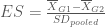
where  = mean of the group G1;  = mean of the group G2; and  is the pooled standard deviation which follows the next formula:

                                                         

being = sample size for G1; = sample size for G2; = the standard deviation of G1; = the standard deviation of G2;

But, how can it be interpreted? Firstly, it can be understood as an index of clinical relevance. The larger the effect size, the larger the difference between groups and the larger the clinical relevance of the results. As it is a quantitative value, ES can be described as small, medium and large effect size using the cut-off values of 0.2, 0.5 and 0.80.
Clinical relevance is commonly assessed as a result of an intervention. Nevertheless, it can be also extended to any other non experimental study design types, for instance, for cross-sectional studies.
To sum up, both significances (statistical and clinical) are not mutually exclusive but complementary in reporting results of clinical research. Researchers should abandon the only use of the p-value interpretation. Here you have a starting point for the evaluation of the clinical relevance.

[1] Cohen J. The concepts of power analysis. In: Cohen J. editor: Statistical power analysis for the behavioral sciences. Hillsdale, New Jersey: Academic Press, Inc: 1998. p. 1-17.

Interview with…..

  Arantzazu Arrospide

 Arantzazu Arrospide Elgarresta studied mathematics in the University of the Basque Country (UPV/EHU) and works as a biostatistician in the Research Unit of Integrated Health Organisations in Gipuzkoa. This research unit gives support to four regional hospitals (about 100 beds each one) and all the public Primary Care Health Services in Gipuzkoa.

Email: arantzazu.arrospideelgarresta@osakidetza.net

and

Irantzu Barrio

  Acting teacher at the Department of Applied  Mathematics, Statistics and Operational Research of the    University of the Basque Country (UPV/EHU)

 Email: irantzu.barrio@ehu.es

 

Both young biostatisticians are currently working on several ongoing research projects. They belong to the Health Services Research on Chronic Patients Network (REDISSEC) – among others  biostatisticians – and tell us what they think about Biostatistics.

1.    Why do you like Biostatistics?

Irantzu Barrio: On one hand I like applying statistics to real problems, data sets and experiments. On the other hand, I like developing methodology which can contribute to get better results and conclusions in each research project. In addition, I feel lucky  to work in multidisciplinary teams. This allows me to learn a lot from other areas and constantly improve on mine own, always looking for ways to provide solutions to other researchers needs.

Arantzazu Arrospide: I think Biostatistics is the link between mathematics and the real world, giving us the opportunity to feel part of advances in scientific research.

2.    Could you give us some insight in your current field of research?

AA: Our main research line is the application of mathematical modeling the evaluation of public health interventions, especially economic evaluations. Although Markov Chain models are the most common methods for this kind of evaluations we work with discrete event simulation models which permit more flexible and complex modeling.

IB: I’m currently working on my PhD thesis. One of the main objectives of this work is to propose and validate a methodology to categorize continuous predictor variables in clinical prediction model framework. Specifically we have worked on logistic regression models and Survival Models.

3.    You have been doing an internship abroad. What was the aim of your stay?

IB: I did an internship in Guimaraes at the University of Minho, Portugal. During my stay, I worked together with Luis Filipe Meira Machado and María Xosé Rodriguez-Alvarez. The aim was to learn more about survival models and extend the methodology developed so far, considering different prediction models.

AA: I did a short stay in the Public Health department of the Erasmus Medical Centre in Rotterdam (Netherlands) last November. The aim of the visit was to discuss the validation of a discrete event simulation model developed to estimate the health effects and costs of the breast cancer screening program in the Basque Country.

4.    What did allow you to do that was has not been possible in Spain?

IB: Oh! It’s amazing when you realize you have all your time to work on your research project, one and a unique priority for more than two months. Of course, all the other to do’s did not disappeared from my calendar, only were postponed until my return to Bilbao. And, in addition to that, it was also a privilege to work together with high experienced biostatisticians and to have the opportunity to learn a lot from them.

AA: The research group I visited, internationally known as the MISCAN group, is the only European member of the Cancer Intervention and Surveillance Modeling Network (CISNET) created by the National Cancer Institute in the United States. Their main objective is to include modeling to improve the understanding of the impact of cancer control interventions on population trends in incidence and mortality. These models then can project future trends and help determine optimal control strategies. Currently, Spanish screening programs evaluation is mainly based on the quality indicators recommended by the European Screening Guidelines which do not include a comparison with an hypothetical or estimated control group.

5.    Which are the most valuable aspects to highlight during your internship? What aspects do you believe that might be improved?

IB: I would say that my internship was simply perfect. When I came back to Bilbao I just thought time had gone really really fast. I’m just looking forward to go back again.

AA: This group works for and in collaboration with their institutions. They are the main responsible of evaluation of ongoing screening programs, prospective evaluation of screening strategies and leaders for new randomized trials in this topic. This is the reference group in the Netherlands for cancer screening interventions and their institutions consider their conclusions when making important decisions.

6.    What do you think of the situation of young biostatisticians in Spain?

AA: When you work in a multidisciplinary research group both methodological and disease specific knowledge are essential and it takes a long time to achieve it. Institutional support is necessary to obtain long term funds that would ensure future benefits in healthcare research based on rigorous and innovative methods.

IB: I think the situations for young biostatisticians and for young people in general is not easy right now. And at least for what I see around me, there is lot of work to do for.

7.    What would be the 3 main characteristics or skills you would use to describe a good biostatistician? And the main qualities for a good mentor?

AA: Open minded, perfectionist and enthusiastic. As for the mentor, he/she  should be strict, committed and patient.

IB: In my opinion good skills on statistics, probability and mathematics are needed. But at the same time I think it is important to be able to communicate with other researchers such as clinicians, biologists, etc, specially to understand which are their research objectives and be able to translate bio-problems to stat-problems.

For me it is very important to have good feeling and confidence with your mentor. I think that having that, everything else is much easier. On the other hand, if I had to highlight some qualities, I would say that a good mentor would: 1) Contribute with suggestions and ideas 2) Supervise the work done and 3) be a good motivator.

8.    Finally, is there any topic you would like to see covered in the blog?

IB: I think the blog is fantastic, there is nothing I missed in it. I would like to congratulate all the organizing team, you are doing such a good job!!! Congratulations!!!

AA: Although it is not considered part of statistical science operational research methods also can be of interest in our researches.

Selected publications (6):

Arrospide, A., C. Forne, M. Rue, N. Tora, J. Mar, and M. Bare. “An Assessment of Existing Models for Individualized Breast Cancer Risk Estimation in a Screening Program in Spain.”. BMC Cancer 13 (2013).

Barrio, I., Arostegui, I., & Quintana, J. M. (2013). Use of generalised additive models to categorise continuous variables in clinical prediction. BMC medical research methodology, 13(1), 83.

Vidal, S., González, N., Barrio, I., Rivas-Ruiz, F., Baré, M., Blasco, J. A., … & Investigación en Resultados y Servicios Sanitarios (IRYSS) COPD Group. (2013). Predictors of hospital admission in exacerbations of chronic obstructive pulmonary disease. The International Journal of Tuberculosis and Lung Disease, 17(12), 1632-1637.

Quintana, J. M., Esteban, C., Barrio, I., Garcia-Gutierrez, S., Gonzalez, N., Arostegui, I., Vidal, S. (2011). The IRYSS-COPD appropriateness study: objectives, methodology, and description of the prospective cohort. BMC health services research, 11(1), 322.

Mar, J., A. Arrospide, and M. Comas. “Budget Impact Analysis of Thrombolysis for Stroke in Spain: A Discrete Event Simulation Model.”. Value Health 13, no. 1 (2010): 69-76.

Rue, M., M. Carles, E. Vilaprinyo, R. Pla, M. Martinez-Alonso, C. Forne, A. Roso, and A. Arrospide. “How to Optimize Population Screening Programs for Breast Cancer Using Mathematical Models.”.

Mixed Models in Sports and Health

As in many other research areas, mixed models have become widely applied in sports science and related health issues. Within sports science, different branches account for the interests of different stakeholders; general managers, coaches, teams, supporters, scientists, academics. Human performance and medicine (treatment and prevention of injuries) lie behind them all and these models are a way to account for within subject variability, time-dependent covariates, and nested data.

On the competition side, efforts have been made in the literature to find ways to model player performance. Casals and Martínez (2013) approach this problem in the context of the NBA basketball league results by considering a balanced design where player is the random intercept and the forward stepwise approach to model selection by Pinheiro and Bates (2000) has been adopted to determine additional factors to be included in the final model. The great advantage of their proposed models for points and win scores over previous studies is that they account for the variation in players´ characteristics and therefore can predict potential variation in player performance using Linear Mixed Models (LMM) and Generalized Linear Mixed models (GLMM), and are consequently of great help for coaches, managers and other decision makers.

A similar methodology has been followed to predict scoring ability in the English football Premier League by McHale and Szczepański (2014). You may recall the post by Hèctor Perpiñán on calculating results probabilities via simulation. While in Perpiñán´s study only teams´ results were considered for the calculations, McHale and Szczepański´s mixed modelling approach allows for the inclusion of players´ ability to create and convert shots as a disaggregated factor from chance. The accuracy in the prediction of their models in this paper shows again the relevance of models that allow the inclusion of players´ characteristics (rather than just teams´).

Of particular note to our readers is the trend towards the implementation of mixed models in open source software exemplified in the aforementioned papers which use R (R Core Team, 2012) for their modelling, in particular packages nlme and lme4. 

In community exercises for promoting physical activity like the one described in Okely et al. (2011), one research aim has been to determine policies and interventions that help to encourage exercising during adolescence in order to alleviate risk factors in the long run. This particular school-based randomised controlled trial used mixed models to account for the hierarchical structure of the data (32 schools from four geographical regions). According to the authors, one of the greatest advantages of the methodology is that it “incorporates all available data allowing for the analysis of partial datasets created when a participant drops out of the study or misses a study visit.”

Moving on to health applications, injury prediction, for instance in baseball pitchers and athletes, can be modelled by deploying similar approaches to determine the existence of statistically significant differences between groups and within days post-injury for example.

Finally, in veterinary epidemiology mixed modelling has become equally mainstream, as discussed in a recent article by Stryhn and Christensen (2014). As an example of an application, animal risk factors associated with health disorders in sport can also be modelled via these techniques. Visser et al. (2013) have studied the effect in race horses in the Netherlands via a cross-sectional study and have considered a random farm effect. Commercial software has been used in these two previous examples. – SAS (PROC MIXED) and GenStat (GLMM)- which are again of common use in the application of mixed models.

As stated by Casals and Martínez (2013), phenomena like Moneyball have raised the profile of sports data analysis. For researchers, big data and more widely, the intrinsic complex structure of the data coming from the aforementioned fields –and I would add software availability- have stimulated application of these types of models and they seem to be here to stay…

These are some of the examples that we have found but we will sure be missing some other very interesting ones so please let us know…Are you a researcher in the area and would like to tell us about your experience? Have you used this sort of model in this or other areas and are you willing to share your experience? 

Main references:

Casals, M., & Martinez, J.A. (2013). Modelling player performance in basketball through mixed models Journal of Performance Analysis in Sport, 13 (1), 64-82

McHale, I., & Szczepański, L. (2014). A mixed effects model for identifying goal scoring ability of footballers Journal of the Royal Statistical Society: Series A (Statistics in Society), 177 (2), 397-417 DOI: 10.1111/rssa.12015

Okely, A., Cotton, W., Lubans, D., Morgan, P., Puglisi, L., Miller, J., Wright, J., Batterham, M., Peralta, L., & Perry, J. (2011). A school-based intervention to promote physical activity among adolescent girls: Rationale, design, and baseline data from the Girls in Sport group randomised controlled trial BMC Public Health, 11 (1) DOI: 10.1186/1471-2458-11-658

Visser, E., Neijenhuis, F., de Graaf-Roelfsema, E., Wesselink, H., de Boer, J., van Wijhe-Kiezebrink, M., Engel, B., & van Reenen, C. (2013). Risk factors associated with health disorders in sport and leisure horses in the Netherlands Journal of Animal Science, 92 (2), 844-855 DOI: 10.2527/jas.2013-6692

Interview with…Manuel G. Bedia

Manuel G. Bedia is an assistant professor in the Department of Computer Science at the University of Zaragoza. He is one of the founders of the Spanish Network of Cognitive Science (retecog.net). This network has been established to promote and coordinate research in Cognitive Systems with goals overlapping those of the European Network EUCognition but with more emphasis on the relationships between scientific and educational policies, and the Spanish university system. He holds a BSc in Physics, a MSc.in Technological Innovation management and a Ph.D. in Computer Science and Artificial Intelligence (Best PhD Thesis Award, 2004), all from the University of Salamanca (Spain). He has worked as a Technological Consultant in Innovation and knowledge management (Foundation COTEC, Madrid, Spain) and as a research fellow in the field of artificial cognitive systems in the Department of Computer Science at the University of Salamanca, the Planning and Learning Group at the University Carlos III of Madrid (Visiting Professor, 2005-07) and the Multidisciplinary Institute at the University Complutense of Madrid (2004-07). He has also been a visiting postdoctoral researcher at the Institute of Perception, Action and Behavior (University of Edinburgh, 2005) and the Centre for Computational Neuroscience and Robotics at the University of Sussex, 2008.

1.     Your area of research is Cognitive Sciences. Could you give us a brief introduction about the focus of your work? 

Cognitive science is a space for interdisciplinary research where we aim to understand how the mind works. It joins together neuroscientists, psychologists, philosophers, engineers and of course statisticians too!

During the past five decades, analogies between the human mind/brain and computer software/hardware have led the work of researchers trying to understand how we think, reason and solve problems.

However, over the last few years, new conceptions have arisen doubting this conceptualisation. The biggest influence behind this change in perspective has come from engineers rather than scientists; in particular a group of engineers using the disciplinary tools of engineering to generate new scientific hypotheses instead of applying knowledge generated from other areas.

In a reversal of the usual role of engineers using models for the development of artifacts, the process develops tools to think about mind phenomena.

2. Could you give us an example of this?

Imagine we purposefully build a very simple artifact or software program that is capable of performing a certain task in a novel way. This proves the existence of explanatory alternatives to phenomena that were supposed to work in a certain way. In the words of other authors, the models serve as “mental gymnastics”. They are entities equivalent to classical mental experiments: They are artifacts that help our thinking. These tools are the foundations of modelling exercises: dynamic systems, probability theory, etc.

3. Is probability an important tool in your work?

It is indeed very important and relevant at many levels of the research in this area.

At a fundamental level, the mathematical languages that the early Artificial Intelligence (AI) researchers developed were not sufficiently flexible (they were based on the use of logic and rule systems) to capture an important characteristic of our intelligence: its flexibility to interactively reorganise itself. This led to a growing interest in tools that would embrace this uncertainty.

Recently a very interesting approach has been developed in the area where fundamental principles are based on probability: Artificial General Intelligence (AGI). The original goal of the AI field was the construction of “thinking machines” – that is, computer systems with human-like general intelligence. Due to the difficulty of this task, for the last few decades, the majority of AI researchers have focused on what has been called “narrow AI” – the production of AI systems displaying intelligence regarding specific, highly constrained tasks. In recent years, however, more and more researchers have reapplied themselves to the original goals of the field recognising the necessity and emergent feasibility of treating intelligence holistically. AGI research differs from the ordinary AI research by stressing the versatility and entirety of intelligence. Essentially, its main objective was to develop a theory of Artificial Intelligence based on Algorithmic Probability (further explanations can be found here).

At a more concrete level, there are several examples. For instance, it is well known that the reasoning model of the clinical environment is fundamentally Bayesian. The clinicians analyse and reflect on previous conditions and status of patients, before reaching a diagnosis of their current condition. This fits very well with the whole idea of Bayesian probability. Following the same line of reasoning, probability appears as a fundamental tool to model artificial minds thinking as humans.

In general, this Bayesian framework is the most used in our field.

4. How can this be applied in your area of research?

The Bayesian framework for probabilistic inference provides a general approach to understanding how problems of induction can be solved in principle, and perhaps how they might be solved in the human mind. Bayesian models have addressed animal learning , human inductive learning and generalisation, visual perception, motor control, semantic memory , language processing and acquisition , social cognition, etc.

However, I believe that the most important use comes from the area of neuroscience.

5. So what is the neuroscientific viewpoint in the field of the understanding of our mental functions, the Cognitive Sciences?

Neuroscience intends to understand the brain from the neural correlates that are activated when an individual performs an action. The advances in this area over the years are impressive but this conceptual point of view is not without problems. For instance, as Alva Noë states in his famous book Out of Our Heads, the laboratory conditions under which the measurements are taken substantially affect the observed task…This is a sort of second order cybernetics effect as defined by Margaret Mead decades ago. The history of neuroscience also includes some errors in the statistical analysis and inference phases…

6. Could you explain this further?

In the early 90s, David Poeppel, when researching the neurophysiological foundations of speech perception, found out that none of the six best studies of the topic matched his methodological apparatus (read more here).

Apparently, these issues were solved when functional magnetic resonance imaging (fMRI) emerged. As this technique was affordable it allowed more groups to work on the topic and indirectly forced the analytical methods to become more standardised across the different labs.

However, these images brought in a new problem. In an article in Duped magazine Margaret Talbot described how the single inclusion of fMRI images in papers had arguably increased the probability of these being accepted.

7.  You have also mentioned that big mistakes have been identified in the statistical analysis of data in the area. What is the most common error in your opinion?

In 2011 an eye-opening paper was published on this topic (find it here). The authors focused their research on the misreported significance of differences of significance.

Let’s assume one effect is statistically significantly different from controls (i.e. p<0.05), while another is not (p>0.05). On the surface, this sounds reasonable, but it is flawed because it doesn’t say anything about how different the two effects are from one another. To do this, researchers need to separately test for a significant interaction between the two results in question. Nieuwenhuis and his co-workers summed up the solution concisely: ‘…researchers need to report the statistical significance of their difference rather than the difference between their significance levels.’

The authors had the impression that this type of error was widespread in the neuroscience community. To test this idea, they went hunting for ‘difference of significance’ errors in a set of very prestigious neuroscience articles.

The authors analysed 513 papers in cognitive neurosciences in the five journals of highest impact (Science, Nature, Nature Neuroscience, Neuron and The Journal of Neuroscience). Out of the 157 papers that could have made the mistake, 78 use the right approach whereas 79 did not.

After finding this, they suspected that the problem could be more generalised and went to analyse further papers. Out of these newly sampled 120 articles on cellular and molecular neuroscience published in Nature Neuroscience between 2009 and 2010, not a single publication used correct procedures to compare effect sizes. At least 25 papers erroneously compared significance levels either implicitly or explicitly.

8. What was the origin of this mistake?

The authors suggest that it could be due to the fact that people are generally tempted to attribute too much meaning to the difference between significant and not significant. For this reason, the use of confidence intervals may help prevent researchers from making this statistical error. Whatever the reasons behind the mistake, its ubiquity and potential effect suggest that researchers and reviewers should be more aware that the difference between significant and not significant events is not itself necessarily significant.

I see this as a great opportunity and a challenge for the statistical community, i.e., to contribute to the generation of invaluable knowledge in the applied areas that make use of their techniques.

Selected publications:

Bedia, M. & Di Paolo (2012). Unreliable gut feelings can lead to correct decisions: The somatic marker hypothesis innon-linear decision chains. FRONTIERS IN PSYCHOLOGY. 3 – 384, pp. 1 – 19 pp. 2012. ISSN 1664-1078

Aguilera, M., Bedia, M., Santos, B. and Barandiaran, X. (2013). The situated HKB model: How sensorimotor spatialcoupling can alter oscillatory brain dynamics. FRONTIERS IN COMPUTATIONAL NEUROSCIENCE. 2013. ISSN 1662-5188

De Miguel, G and Bedia, M.G. (2012). The Turing Test by Computing Interaction Coupling. HOW THE WORLD COMPUTES: TURING CENTENARY CONFERENCE AND 8TH CONFERENCE ON COMPUTABILITY IN EUROPE, CIE 2012. Cambridge, ISBN 3642308694

Santos, B., Barandiaran, X., Husband, P., Aguilera, M. and Bedia, M. (2012). Sensorimotor coordination and metastability in a situated HKB model. CONNECTION SCIENCE. 24 – 4, pp. 143 – 161. 2012. ISSN 0954-0091

Spatial objects in R (I)

In this post I would like to offer a brief and practical introduction to different types of spatial data that we could handle in R and how to do to access and visualize them. It might be interesting for those who are beginners in spatial analysis.

The structure of spatial objects is complex, and it is very important to know how these are stored and organized. sp package provides a clear form to organize the spatial data through classes (to specify the structure ) and methods (particular functions for a special data class).

The basic type of spatial objects is Spatial class, in which we could recognize two principal components, called slots: the first one is a bounding box that contains a matrix with the coordinate values. The second is a CRS class object, the reference system for these coordinates (“longlat” for geographical coordinates, “utm” for UTM coordinates, ect). With the command getClass(“Spatial”) (once sp package has been installed), we can examine the different types of spatial objects and their subclasses.

I will use an example to make this something practical, specifically we use a Spanish cartography (“ESP_adm.zip”, downloaded in this web site: http://www.gadm.org/). To use the ‘readShapeSpatial’ function to read the .shp object, we need the library ‘maptools’.

library(maptools)
# load the shapefile:
map <- readShapeSpatial('ESP_adm2.shp')
# map is a SpatialPolygonsDataFrame, a subclass of a SpatialPolygons object.

 A Spatial Polygons object is a closed line, a sequence of point coordinates where the first point is the same as the last point. It is not easy to know their structure, let us look at this briefly:

# examine the structure of this SpatialPolygonsDataFrame object.
# Each slot (5) is determined by ‘@name_slot’
str(map, max.level = 2)

But, what means each slot?

• @data: a data frame which contains information about each polygon. (For instance, the name of provinces, autonomous community,…). To access:

# The provinces:
map@data$NAME_2 # or slot(map, ‘data’)$NAME_2
# Idem for autonomous community with ‘$NAME_1’

• @polygons: a list of 51 polygons (all provinces), of class Polygon. Each of those polygons have 5 slots, we can see the structure of the first polygon with:

   str(map@polygons[[1]]@Polygons) 

• @plotOrder: a vector of the plotting order of the 51 polygons.
• @bbox: two-dimensional matrix with the maximum and minimum of the coordinates.
• @proj4string: the coordinate reference system (CRS class).

Finally, I will give just a simple example of how to plot some geographical coordinates in the ‘map’. For this, we read a data file with the locations and associate a spatial structure creating a SpatialPoints class.  We need to be careful with the reference system of the SpatialPolygons and the SpatialPoints we used. The coordinate reference system for our shapefile is latitude/longitude and the WGS84 datum. Thus, we need the same CRS to our SpatialPoints. But…what if we do not have geographic coordinates? Let’s see it!

Assume that the coordinate reference system of the SpatialPoints is UTM (Universal Transverse Mercator) instead of latitude/longitude.

loc_utm <- read.csv(“loc_utm.csv”,header=T)

> loc_utm
X       Y
1  718970.0 4376275.0
2 505574.2 4793683.2
3  276066.1 4542666.9
4  538135.4 4750010.9

There are four locations situated (in order) in Valencia, Bilbao, Salamanca and Santiago de Compostela. The first three points are in UTM zone 30 and the last one in zone 29. It is important to know this to define the CRS correctly:

# We separate these points according to the zone:
loc1 <- loc_utm[1:3,]
loc2 <- loc_utm[4,]

# To create a SpatialPoints:
coordinates(loc1) <- c("X","Y")
coordinates(loc2) <- c("X","Y")

# To define the CRS:
proj4string(loc1) <- CRS("+proj=utm +zone=30 +ellps=WGS84")
proj4string(loc2) <- CRS("+proj=utm +zone=29 +ellps=WGS84")

# spTransform function provide transformation between projections.
library(rgdal)
loc1_geo<- spTransform(loc1, CRS("+proj=longlat +ellps=WGS84"))
loc2_geo<- spTransform(loc2, CRS("+proj=longlat +ellps=WGS84"))

Now we can plot these points over the Spanish mapping.

plot(map)
plot(loc1_geo,add=T)
plot(loc2_geo,add=T)

This post has been a short summary of some of Spatial objects that we can manipulate in R. In the following posts I will invite you to continue learning about this area of statistics. I hope it helps someone!

Working with Joint Models in R

Following previous posts on longitudinal models (see posts) and interviews where mentions have been made to survival analysis (read one of these interviews), we will focus today on models incorporating both methodologies, the so-called Joint Models.

Often problems pose more than a single approach. For example, when HIV data are analyzed, we can on the one hand focus on studying the evolution of CD4 cell counts (longitudinal model) and on the other hand, we can also study the time to death (survival analysis model). Joint modeling will allow both models to share information and will achieve better results.

From a practical point of view, in R, we can use two packages called JM and JMbayes to fit these models, under either the frequentist or the Bayesian paradigm, respectively. The use of these packages is not difficult because they are based on the use of packages nlme and survival with which you might already be familiar.

Here I show you how to use them:

• We loaded packages JM and JMbayes

library(JM)
library(JMbayes)

• We fit the longitudinal and survival models independently, saving the results in objects

# Fit the longitudinal model
lmeFit.aids <- lme(CD4 ~ obstime * drug, random = ~obstime | patient, data = aids)
# Fit the survival model
survFit.aids <- coxph(Surv(Time, death) ~ drug, data = aids.id, x = TRUE)

• We use the objects lmeObject and survObject with the functions in the packages JM and JMbayes

# Fit the joint model (Frequentist)
jointFit.aidsFREQ <- jointModel(lmeFit.aids, survFit.aids, timeVar = "obstime")
# Fit the joint model (Bayesian)
jointFit.aidsBAYES <- jointModelBayes(lmeFit.aids, survFit.aids, timeVar = "obstime")

It’s possible to specify different characteristics about the joint model. With JM package various options for the survival model are available. With JMbayes it is possible to choose the type of association structure between the longitudinal and survival processes.

Finally, if you are interested in these models and are thinking about using them in your research, a good reference is the book Joint Models for Longitudinal and Time-to-Event Data: With Applications in R of Dimitris Rizopoulos, author of JM and JMbayes.

Note: The databank to fit the longitudinal model must have as many rows as observations per patient have (aids). On the other hand, the survival model requires a database that has only one observation for each patient over time to death and censoring indicator (aids.id).

Have an animated 2014!

Animations can be a refreshing way to make a website more attractive, as we did exactly a year ago here.

Based on the Brownian motion simulated here, and using animation and ggplot2 R packages, we produced a fun welcome to the International year of Statistics, Statistics2013. The function saveMovie (please notice that there exists another alternative, saveGIF) allowed us to save it and finally publish it, as easy as that!

 
 
 
 
 
 
 
 
 
 
For this new year we have based our work on the demo(‘fireworks’) from the 2.0-0 version of the package animation (find  here a list of the changes in each version) and world from the package maps (speaking of maps, have a look at this great dynamic map by Bob Rudis!).

They also come very handy when trying to represent visually a dynamic process, the evolution of a time-series,etc.

As an example, in a previous post we  portrayed an optimisation model in which the values for the mean were asymptotically approaching the optimal solution, which was achieved after a few iterations. This was done with a for loop and again packages ggplot2 and animation.

There are many other examples of potential applications both in general Statistics – see this animated representation of the t distribution and these synchronised Markov chains and posterior distributions plots– and  in Biostatistics. Some examples of the latter are this genetic drift simulation by Bogumił Kamiński and this animated plots facility in Bio7, the integrated  environment for ecological modelling.

R package caTools also allows you to read and write images in gif format.

Finally, in LaTeX, \animategraphics from the animate package will do the trick; check this post by Rob J. Hyndman for further details.

It is certainly one of our new year’s resolutions to incorporate more animations in our posts, what are yours?

Interview with… Anabel Forte

Anabel Forte Deltell, graduated in mathematics and statistics, holds a PhD in Statistics from the Univeristy of Valencia. Now she is a lecturer at the economics department of Universitat Jaume I at Castellón. Her research topics cover many fields of statistics as, for instance, spatial analysis or joint modeling of longitudinal (or panel) data and time-to-event data with her main interest beeing Bayesian model selection and, in particular, Objective Bayesian variable selection. Her dissertation (2011) entitled “Objective Bayes Criteria for Variable Selection” focuses on this last topic. She has published various articles in international journals and participated in many national and international meetings.

Email: forte@uji.es

 1.   Why do you like Biostatistics?

Researching in biostatistics is researching in real life and it makes me feel like I’m helping to improve people´s life conditions.

 2. Could you give us some insight in your current field of research?

Despite my main line of research being Bayesian model selection, I’m actually working in joint modeling of longitudinal data and time-to-event data. Nowadays many practitioners are moving to what it is called personalized medicine with medical decisions, practices, and/or products being tailored to the individual patient. In this scenario longitudinal data seems to be of great importance since it allows for the consideration of several sources of uncertainty including patient-specific variability. Moreover, quantifying the risk of suffering a certain event of a patient given its trajectory seems really sensible and can be done using joint modeling.

 3. Which are, in your opinion, the main advantages of being a researcher?

For me, being a researcher is simply a way of life. I can not imaging myself doing anything else.

 4. Your whole professional experience has been within the public sector and the University. How do you see the present and future of research in the Spanish public sector?

From my point of view if things do not change greatly, researching in Spain, at least in the public sector, has a really black future. As I see it, the only way researchers can manage to get money is to call attention of private investors. But private money can compromise the objectivity of research and at the same time avoid researching in some fields that are not so “attractive” for industry. Hence it is something that has to be studied carefully… but something has to be done, that´s for sure.

 5. What do you think of the situation of young biostatisticians in Spain?

As I see it, young biostatisticians have to make a great effort to show their enormous value for private companies as, for instance, food processing companies or health care related companies among others… And I think so because, pitifully, nowadays the Spanish public system can not assume all the biostatistical research that is needed.

 6. What would be the 3 main characteristics or skills you would use to describe a good biostatistician?

For me it is really important to have a good mathematical/probabilistic base and to be well organized when working. But the most important of all is enjoying research.

 7. Which do you think are the main qualities of a good mentor?

For me, a good mentor is someone that supervises your work and is always there for you but at the same time he or she should give you some space for you to fail and learn… in other words someone that teaches you what researching really is.

Selected publications:

• Francisco Pozo-Rodríguez; Jose Luis López-Campos; Carlos J. Álvarez-Martínez; Ady Castro-Acosta; Ramón Agüero; Javier Hueto; Jesús Hernández-Hernández; Manuel Barrón; Victor Abraira; Anabel Forte; Juan Miguel Sanchez Nieto; Encarnación Lopez-Gabaldón; Borja G. Cosío; Alvar Agusti. Clinical Audit of COPD patients requiring hospital admissions in Spain: AUDIPOC Study.Plos One. 7 – 7, (USA): 2012.
• M. J. Bayarri; J. O. Berger; A. Forte; G. García-Donato. Criteria fo Bayesian model choice with application to variable selection. Annals of Statistics. 40 – 3, pp. 1550 – 1577. (USA): 2012.
• C. Armero; A. Forte; A. López-Quílez. Geographical variation in pharmacological prescription. Mathematical and Computer Modelling. 50, pp. 921 – 928. (UK): 2009.
• Allepuz; A. López-Quílez; A. Forte; G. Fernández; J. Casal. Spatial Analysis of Bovine Spongiform Encephalopathy in Galicia, Spain (2000-05). Preventive Veterinary Medicine. 79 – 2, pp. 174 – 185. (Holland): 2007.
• López-Quílez; C. Armero; A. Forte. Geographical variation of Pharmacological prescription with Bayesian Hierarchical models.Value In Health. 10 – 6, (USA): 2007.

Hasta la vista, Statistics2013!

After twelve months filled with exciting events celebrating the great role of statistics in society, it is now time to say goodbye to the International Year of Statistics, Statistics2013.

Illustration: Cinta Arribas

From FreshBiostats we would like to thank the steering committee for making of this such a fantastic opportunity for professionals and students at all levels to interact and share the pride in what we do. We would like to send a special thank you to Ronald Wasserstein and Jeffrey Myers who helped us feel involved in the celebration with our small contributions to their newsletter and blog.

The good news is that it seems like there will be a new project starting in late January. We are really looking forward to The World of Statistics! – find here a whole lot of new activities already arranged for 2014-.

How to make an R package repository: an R-recipe

It is well known that R is one of the most used statistical package by the data scientists (researchers, technicians, etc..). This package allows flexibility to adapt already developed functions to their own interests. However, the problem comes when one needs to perform a complex algorithm that requires strong programming level or even to show to worldwide scientists how a new statistical technique works. When this scenario is present, it means that it is time to create your own package in R.

The most In this post we will learn how to make a simple R package only following several steps which are explained in the next paragraphs:

1. Update R version and other relevant tools.

First of all, if you are planning to develop a R package, it is highly recommended to update your R version to newest one. One must take into account that R versions are continuously updating so that your package would be likely to not to work properly. Furthermore, the package called Rtools is necessary to install in your system. This package has several add-ins (such as MinGW compiler) which are helpful for the development of the package.

2. Get to know your Operative System

For Windows System, you have to add to the PATH system variable the whole path where R is installed. For instance, if R is installed in c:, the PATH can be fixed as:

PATH=%PATH%;c:\Rtools\bin;c:\Rtools\perl\bin;c:\Rtools\MinGW\bin;

c:\texmf\miktex\bin;c:\R-2.15.0\bin;

3. Decide the name and the kind of the package wanted to build.

This step is the most important. First of all, the package name can only be composed by numbers and letters and it is highly recommended to start it with a letter.

When building the functions belonging to the package, it is very important the arrangement of the files where the functions are written. There are two possible situations: (1) all functions in a file; (2) each function in its own file.  Both options are extreme since (1) writing all functions in a file could overload the system and (2) writing many functions in its own files implies having multiple files that should be packed. So, in order to search an alternative to these options, I suggest grouping related functions into the same files.

4. Edit some files

Once the previous steps are done, several files should be filled out/edited so that any R user who wants to use the functions within the package is able to understand what the function does.

First of all, it is obligatory to fill in  a file named DESCRIPTION. It is used to describe the package, with author, and license conditions in a structured text format that is readable by computers and by people.

Secondly, a tutorial of the package (called as VIGNETTES) should be written. An extended description with reproducible examples  shows the performance of each function within the repository.

5. Building, installing and executing the package

As final step, you have to mix all the components in a file by means of different software commands. Using the package.skeleton() function (see below) one can create the desired mypkg package:

package.skeleton(list=c(“f”,”g”,”h”,”i”),name=”mypkg”)

where f, g, h, i¸ are all the functions belonging to the repository.

Once mypkg is created, the next step is to install it in our R system. You can use the common ways to perform it but I would advise using R commands to do that (R CMD INSTALL). Load the package and execute it. It is time to enjoy it!!

This has been a summary of the steps to follow for a R package repository development. Now it is your challenge!!!

Merry Christmas and Happy New Year!

Analysis of PubMed search results using R

Looking for information about meta-analysis in R (subject for an upcoming post as it has become a popular practice to analyze data from different Genome Wide Association studies) I came across  this tutorial from The R User Conference 2013 – I couldn´t make it this time, even when it was held so close, maybe Los Angeles next year…

Back to the topic at hand, that is how I found out about the RISmed package which is meant to retrieve information from PubMed. It looked really interesting because, as you may imagine,this is one of the most used resources in my daily routine.

Its use is quite straightforward. First, you define the query and download data from the database (be careful about your IP being blocked from accessing NCBI in the case of large jobs!) . Then, you might use the information to look for trends on a topic of interest or extracting specific information from abstracts, getting descriptives,…

In order to try it out, I decided to get data regarding what has been published relating to Next Generation Sequencing. For doing so, I adopted the search terms proposed in the paper by Jia et al. Through the following code we can get the PubMed results for these search terms since 1980:

library(RISmed)
query = "(exome OR whole OR deep OR high-throughput OR (next AND generation) OR (massively AND parallel)) AND sequencing"
ngs_search <- EUtilsSummary(query, type="esearch",db = "pubmed",mindate=1980, maxdate=2013, retmax=30000)
QueryCount(ngs_search)
ngs_records <- EUtilsGet(ngs_search)
years <- Year(ngs_records)
ngs_pubs_count <- as.data.frame(table(years))

This code allow us to get published papers on this topic per year. By getting also data about the total number of publications per year, we are able to normalize the data. The complete R code, once the data are downloaded and edited can be found at  FreshBiostats GitHub Gist. In the next graph, we can see the publication trend for Next Generation Sequencing per year:

I was also curious about which ones would be the journals with the highest number of publications on this topic. Using the following code we can get the count of NGS publications per journal:

journal <- MedlineTA(ngs_records)
ngs_journal_count <- as.data.frame(table(journal))
ngs_journal_count_top25 <- ngs_journal_count[order(-ngs_journal_count[,2]),][1:25,]

Again, the complete code that allows us to normalize the data by the total number of publications per journal, as well as the following barplots showing the result, is available at our Gist:

You cand find some other examples using this package at Dave Tangs Bioinformatics blog. Additionally, some alternatives to the use of RISmed package can be found at R Chronicle and R Psychologist blogs.

Other potential applications of this package include creating a co-author network, as is described in Matthew Maenner´s blog.

Search and analyze carefully!

My impressions from the Workshop on the Future of the Statistical Sciences

An exciting workshop, organised as the capstone of the International Year of Statistics Statistics2013, was celebrated on the 11^th and 12^th of November at the Royal Statistical Society Headquarters in London, under the stimulating title of  “The Future of the Statistical Science”, science to which John Pullinger, president of the Royal Statistical Society, refers to as a quintessentially, multidisciplinary discipline. The workshop was indeed a good example of that.

Online attendance was welcomed to the event giving an additional opportunity to listen to highly reputed professionals in main areas of Statistics. Virtual participants were also allowed to pose their questions to the speakers, an innovation that worked very well as an excellent way to make these sorts of events available to a wider audience that would otherwise be excluded – I am already looking forward to more! -.

In case you missed it at the time, luckily the podcast is still available here.

True to its description, the event covered different areas of application, it showed the tools of the field for tackling a wide range of challenges, it portrayed potentially high impact examples of research, and in summary, was a great attention-grabbing exercise that will hopefully encourage other professionals to the area. A common vision of ubiquity and great relevance came across from the speeches and showed the field as a very attractive world to join. See my simplified summary below in form of a diagram certainly reflective of the great Statistics Views motto “Bringing Statistics Together”.

Fig 1. Some of the ideas discussed in the workshop

Particularly relevant to this blog and my particular interests were presentations on environmental Statistics and statistical Bioinformatics, as well as other health-related talks. Important lessons were taken on board from the rest of the speakers too.

The workshop started with a shared presentation on the hot topic “Statistical Bioinformatics” by Peter Bühlmann (ETH Zürich) and Martin Vingron (Free University of Berlin). In a fascinating talk, Bühlmann argued for the need of uncertainty quantification in an increasingly heterogeneous data world –examples of this are also appearing in other fields, e.g. in the study of autism disorders as Connie Kasari and Susan Murphy mentioned in “SMART Approaches to Combating Autism”- and for models to be the basis of the assignation of uncertainties – topic greatly covered by Andrew Gelman in “Living with uncertainty, yet still learning”-, while acknowledging that in the big data context, “confirmatory statistical inference is (even more) challenging”. Vingron followed by focusing on “Epigenomics as an example”, raising open questions to the audience on how to define causality in Biology where “most processes […] are feedback circular processes”, calling for models that are just complex enough so as to allow for mechanistic explanations, and for good definitions of null hypotheses.

In addition to the interesting points of the talk, I found its title particularly attractive in what it could be directly linked to a vibrant roundtable on “Genomics, Biostatistics and Bioinformatics” in the framework of the 2nd Biostatnet General Meeting, in which, as some of you might remember, the definitions of the terms Biostatistics and Bioinformatics were discussed. I wonder if the term “statistical Bioinformatics” would be indeed the solution to that dilemma? As a matter of fact, Bühlmann himself mentions at the start of his talk other options like Statistical Information Sciences, etc-

Michael Newton and David Schwartz from the University of Wisconsin-Madison also focused on the triumph of sequencing and “Millimeter-long DNA Molecules: Genomic Applications and Statistical Issues”. Breast cancer being one of the mentioned applications, this was followed by an introduction to “Statistics in Cancer Genomics” by Jason Carroll and Rory Stark (Cancer Research UK Cambridge Institute, University of Cambridge), particularly focusing on breast and prostate cancer and the process of targeting protein binding sites.  The latter, as a computational biologist, mentioned challenges on the translation of Statistics for the biologists and vice versa, and identified ”reproducibility as (the) most critical statistical challenge” in the area – also on the topic of reproducibility, it is especially worth watching “Statistics, Big Data and the Reproducibility of Published Research” by Emmanuel Candes (Stanford University) -.

Another area increasingly gaining attention in parallel with technologies improvements is Neuroimaging. Thomas Nichols (University of Warwick) lead the audience in a trip through classical examples of its application (from Phineas Gage´s accident to observational studies of the structural changes in the hippocampi of taxi drivers, and the brain´s reaction to politics) up to current exciting times, with great “Opportunities in Functional Data Analysis” which Jane-Ling Wang (University of California) promoted in her talk.

Also in the area of Health Statistics, different approaches to dietary patterns modelling were shown in “The Analysis of Dietary Patterns and its Application to Dietary Surveillance and Epidemiology” by Raymond J. Carroll (Texas A&M University), and Sue Krebs-Smith (NCI), with challenges in the area being; finding dietary patterns over the life course – e.g. special waves of data would appear in periods like pregnancy and menarchy for women-, and incorporation of technology to the studies as a new form of data collection –e.g., pictures of food connected to databases-.

Again with a focus on the challenges posed by technology, three talks on environmental Statistics outlined an evolution over time of the field. Starting from current times, Marian Scott (University of Glasgow) in “Environment – Present and Future” stated in her talk that “natural variability is more and more apparent” because we are now able to visualise it. This idea going back to the heterogeneity claimed by Bühlmann. Despite the great amounts of data being available, and initially caused by technological improvements but ultimately due to a public demand – “people are wanting what it is happening now”-, the future of the field is still subject to the basic questions: “how and where to sample.” Especially thought-provoking were Scott´s words on “the importance of people in the environmental arena” and the need for effective communication: “we have to communicate: socio-economic, hard science…, it all needs to be there because it all matters, it applies to all the world…”

Amongst other aims of this environmental focus such as living sustainably – both in urban and rural environments-, climate is a major worry/fascination which is being targeted through successful collaborations of specialists in its study and statisticians. “Climate: Past to Future” by Gabi Hegerl (University of Edinburgh) and Douglas Nychka (NCAR) covered “Regional Climate – Past, Present and Future” and showed relevant examples of these successful collaborations.

Susan Waldron (University of Glasgow), under the captivating speech title of “A Birefringent Future”, highlighted the need to address challenges in the communication of “multiple layers of information” too, Statistics appearing as the solution for doing this effectively –e.g. by creating “accessible visualisation of data” and by incorporating additional environmental variation in controversial green energy studies such as whether wind turbines create a microclimate-. Mark Hansen (Columbia University Journalism School) seconded Waldron´s arguments and called for journalists to play an important role in the challenge: “data are changing systems of power in our world and journalists. […] have to be able to think both critically as well as creatively with data”, so as to “provide much needed perspective”. Examples of this role are; terms such as “computational Journalism” already being coined and data visualisation tools being put in place -as a fascinating example, the New York Times´ Cascade tool builds a very attractive representation of the information flow in Social Media-. David Spiegelhalter (Cambridge University) also dealt with the topic in the great talk “Statistics for an Informed Public”, providing relevant examples (further explanation on the red meat example can be found here as well).

To encourage “elicitation of experts opinions (to reach a) rational consensus” and “to spend more time with regulators” came up as other useful recommendations in the presentation “Statistics, Risk and Regulation” by Michel Dacorogna (SCOR) and Paul Embrechts (ETH Zürich).

In a highly connected world inmersed in a data revolution, privacy becomes another major issue. Statistical challenges arising from networked data –e.g. historical interaction information modelling- were addressed by Steve Fienberg (Carnegie Mellon University) and Cynthia Dwork (Microsoft Research), who argued that “statisticians of the future will approach data and privacy (and its loss) in a fundamentally algorithmic fashion”, in doing so explicitly answering the quote by Sweeney: “Computer science got us into this mess, can computer science get us out of it?”. Michael I. Jordan (University of California-Berkeley) in “On the Computation/Statistics Interface and “Big Data”” also referred to “bring(ing)  algorithmic principles more fully into contact with statistical inference“.

I would like to make a final mention to one of the questions posed by the audience during the event. When Paul Embrechts was enquired about the differences between Econometrics and Statistics, a discussion  followed on how crossfertilisation between fields has happened back and forth. As a direct consequence of this contact, fields rediscover issues from other areas. For instance, Credit Risk Analysis models were mentioned as being inferred from Medical Statistics or back in Peter Bühlmann´s talk, links were also found between Behavioural Economics and Genetics. These ideas, from my point of view, bring together the essence of Statistics, i.e. its application and interaction with multiple disciplines as the foundations of its success.

Many other fascinating topics were conveyed in the workshop but unfortunately, I cannot fit here mentions to all the talks. I am sure you will all agree it was a fantastic event.

Setting up your (Linux biostatistical) workstation from scratch

Facundo Muñoz, MSc in Mathematics, PhD in Statistics from University of Valencia. He is currently a postdoc researcher at the french Institute National de la Recherche Agronomique (INRA). His main research field is spatial (Bayesian) statistics applied to environmental and biostatistical problems. He is currently working on statistical methodologies for the analysis of forest genetic resources.

Being a busy biostatistician, I spend plenty of time glued to my computer. As an immediate consequence, every once in a while I need to set up my working station from zero. Either when I change job (I have done twice this year!), or when I want to update my OS version (upgrades rarely go perfect), or when I get a new laptop.

This involves, you know, installing the OS, the main programs I need for work like R and LaTeX, some related software like a good Control Version System, a couple of Integrated Development Environments for coding and writing, and a dozen of other ancillary tools that I use every now and then.

Furthermore, I need to configure everything to run smoothly, set up my preferences, install plugins, and so on.

Last time I did this manually, I spent a week setting everything up, and in the following days I always had something missing. Then I thought I should have got this process scripted.

Last week I set up my working environment in my new job. In a few hours I had everything up and running exactly the way I like. I spent an aditional day updating the script with new software, updated versions, and solving some pending issues.

I thought this script might be useful for others as well, hence this post. It is version-controled in a google code repository, where you can download the main script.

It is not very general, as installation details changes a lot from system to system. I use Linux Mint, but I believe it should go pretty straightforward with any derivative of Ubuntu, or Ubuntu itself (those distros using the APT package management). Other Linux branches (Arch, RedHat, Suse, Mac’s Darwin) users would need to make significant changes to the script, but still the outline might help. If you use Windows, well… don’t.

Of course, you will not be using the same software as I do, nor the same preferences or configurations. But it might serve as a guide to follow line by line, changing things to suit your needs.

In particular, it provides an almost-full installation (without unnecessary language packages) of the very latest LaTeX version (unlike that in the repos), and takes care of installing it correctly. It also sets up the CRAN repository and installs the latest version of R.

The script also installs the right GDAL and Proj4 libraries, which are important in case you work with maps in R or a GIS.

Finally, it installs some downloadable software like Kompozer (for web authoring), the Dropbox application, and more. It scrapes the web in order to fetch the latest and right versions of each program.

I hope it helps someone. And if you have alternative or complementary strategies, please share!

FreshBiostats´ First Anniversary

So here we are. It has been a year since we started this venture. The idea of a blog came up from one of our co-bloggers at the Jede II Conference in the summer of 2012.  At first it sounded like a bit of a challenge, but who said fear?

No doubt about it, the balance has been highly positive. We are all for sharing knowledge and resources that might be valuable for others, and from our humble perspective we sincerely hope it might have been of some use. It has certainly been so for us, both by getting insight into particular subjects when writing the different posts and by diving into new topics covered by our co-bloggers and invited posts. Twitter and facebook have also allowed us to encourage interaction with colleagues and other bloggers, and we can now say our social and professional networks have certainly become bigger and stronger!

We have found it difficult at times to juggle our jobs and PhDs with writing our weekly posts but as we said in several occasions, we are passionate about our work, and firmly believe that, most of the time, the line between work and fun gets blurry.

As we promised in a previous post, here is an infographic summarising this year of Fun & Biostatistics, enjoy!

We have a very international audience with visits coming from 117 countries, and we are delighted to see that not only colleagues from our closest network are reading our entries. Since our participation on the International Statistics Year blog -Statistics2013- and after being mentioned in other blogs such as RBloggers and others, we have gained more visibility and some posts have become very popular (more than 1000 views for some!).

Those posts focusing on R tips clearly take the cake, being the most visited. We guess they might be the most useful ones, as we are also big fans of other very practical blogs. However we like to cover all the aspects of our profession and even sometimes deal with more controversial or philosophical subjects…

We will keep inviting people to share their knowledge and will encourage colleagues to get involved in the blog. Our second year resolution is to make an effort to make of this blog a more interactive tool. We count on you for that!

Remember you can contact us with your comments, suggestions, and enquiries at freshbiostats@gmail.com

Thank you so much for being there!

Interview with…Jorge Arribas

Jorge is a BSc Pharmacy from the UPV-EHU and he is currently a resident trainee in Microbiology and Parasitology at the H.C.U. Lozano Blesa in Zaragoza, working also on his PhD thesis.

Email: Jarribasg(at)salud(dot)aragon(dot)es

 1.     Could you give us some insight in your current field of research?

My PhD thesis focuses on the diagnosis of Hepatitis C Virus (HCV) infection by means of core antigen determination, and I am also collaborating in a line of research focusing on new treatments for H. pylori infection, funded by a FIS grant. The former, intends to perform a comparison with respect to the current technique in use for the diagnosis. The latter, analyses resistance to different Flavodoxin inhibitors.

2.     Where does Biostatistics fit in your daily work?

In both areas of research that I am working on, since they are essentially comparative studies against established techniques, and therefore require techniques to prove the significance – or lack of significance- of the improvements.

3.     Which are the techniques that you or researchers in your area use more often?

Statistical techniques such as sensitivity and specificity analysis, hypothesis testing (ANOVA, t-test). There is also a particular need in the area for techniques dealing with ordinal data.

4.     As a whole, do you find Biostatistics relevant for your profession?

A very important part of the speciality of Microbiology and Parasitology focuses on the research of new diagnostic methods, treatments, prevalence of antibiotic resistance, etc. Therefore, Biostatistics becomes extremely useful when comparing these novel approaches to previous ones.

5.     Finally, is there any topic you would like to see covered in the blog?

It would be great to see published some examples of statistical applications in my area of study.

Selected publications:

• J. Arribas, R. Benito , J. Gil , M.J. Gude , S. Algarate , R. Cebollada , M. Gonzalez-Dominguez , A. Garrido, F. Peiró , A. Belles , M.C. Rubio (2013). Detección del antígeno del core del VHC en el cribado de pacientes en el programa de hemodiálisis. Proceedings of the XVII Congreso de la Sociedad Española de Enfermedades Infeccionas y Microbiología Clínica (SEIMC).
• M. González-Domínguez, C. Seral, C. Potel, Y. Sáenz, J. Arribas, L. Constenla, M. Álvarez, C. Torres, F.J. Castillo (2013). Genotypic and phenotypic characterisation of methicillin-resistant Staphylococcus aureus (MRSA) clones with high-level mupirocin resistance in a university hospital. Proceedings of the 23nd European Congress of Clinical Microbiology and Infectious Diseases and 28th International Congress of Chemotherapy.
• M. González-Domínguez, R. Benito, J. Gil,  MJ. Gude, J. Arribas, R. Cebollada, A. Garrido, MC. Rubio (2012).  Screening of Trypanosoma cruzi infection with a chemiluminiscent microparticle immunoassay in a  Spanish University Hospital. Proceedings of the 22nd European Congress of Clinical Microbiology and Infectious Diseases and 27th International Congress of Chemotherapy.

FreshBiostats birthday and September-born famous statisticians

With the occassion of the 1st birthday of FreshBiostats, we want to remember some of the great statisticians born in September and that have contributed to the “joy of (bio)stats”.

Gerolamo Cardano	Pavia, 24 September 1501 – 21 September 1576	First systematic treatment of probability
Caspar Neumann	Breslau, 14 September 1648 – 27 January 1715	First mortality rates table
Johann Peter Süssmilch	Zehlendorf, 3 September 1707 – 22 March 1767	Demographic data and socio-economic analysis
Georges Louis Leclerc (Buffon)	Montbard, 7 September 1707 – Paris, 16 April 1788	Premier example in “geometric probability” and a body of experimental and theoretical work in demography
Adrien-Marie Legendre	Paris, 18 September 1752 – 10 January 1833	Development of the least squares method
William Playfair	Liff, 22 September 1759 – London, 11 February 1823	Considered the founder of graphical methods of statistics (line graph, bar chart, pie chart, and circle graph)
William StanleyJevons	Liverpool, 1 September 1835 – Hastings,13 August 1882	Statistical atlas – graphical representations of time series
Anders Nicolai Kiaer	Drammen, 15 September 1838 – Oslo, 16 April 1919	Representative sample
Charles Edward Spearman	London, 10 September 1863 – 17 September 1945	Pioneer of factor analysis and Spearman´s Rank correlation coefficient
Anderson Gray McKendrick	Edinburgh, September 8, 1876 – May 30, 1943	Several discoveries in stochastic processes and collaborator in the path-breaking work on the deterministic model for the general epidemic
Maurice Fréchet	Maligny, 2 September 1878 – Paris, 4 June 1973	Contributions in econometrics and spatial statistics
Paul Lévy	15 September 1886 – 15 December 1971	Several contributions to probability theory
Frank Wilcoxon	County Cork, 2 September 1892 – Tallahassee, 18 November 1965	Wilcoxon rank-sum tests, Wilcoxon signed-rank test
Mikhailo Pylypovych Kravchuk	Chovnytsia, 27 September 1892- Magadan, 9 March 1942	Krawtchouk polynomials, a system of polynomials orthonormal with respect to the binomial distribution
Harald Cramér	Stockholm, 25 September 1893 – 5 October 1985	Important statistical contributions to the distribution of primes and twin primes
Hilda Geiringer	Vienna, 28 September 1893 – California, 22 March 1973	One of the pioneers of disciplines such as molecular genetics, genomics, bioinformatics,…
Harold Hotelling	Fulda, 29 September 1895 – Chapel Hill, 26 December 1973	Hotelling´s T-squared distribution and canonical correlation
David van Dantzig	Rotterdam, 23 September 1900 -Amsterdam,  22 July 1959	Focus on probability, emphasizing the applicability to hypothesis testing
Maurice Kendall	Kettering, 6 September 1907 – London, 29 March 1983	Random number generation and Kendall´s tau
Pao-Lu Hsu	Peking, 1 September 1910 – Peking, 18 December 1970	Founder of the newly formed discipline of statistics and probability in China

It is certainly difficult to think of the field without their contributions. They are all a great inspiration to keep on learning and working!!

Note: you can find other interesting dates here.

Update: and Significance´s timeline of statistics here.

Any author you consider particularly relevant? Any other suggestions?

Infographics in Biostatistics

Although the history of Infographics according to Wikipedia does not seem to mention Fritz Kahn as one of the pioneers of this technique, I would like to start this post mentioning one of the didactic graphical representations of this Jewish German doctor, who was highly reputed as a popular science writer of his time.

Apart from his fascinating views of the human body in the form of machines and industrial processes, I am particularly attracted by his illustration below, summarising the evolution of life in the Earth as a clock in which the history of humans would not take more than a few seconds…

Image extracted from the printed version of the article “Fritz Kahn, un genio olvidado” published in El País, on Sunday 1st of September 2013.

 What could be understood by some as a naive simplification of matters requires, in my opinion, a great deal of scientific knowledge and it is a fantastic effort to communicate the science behind very complex mechanisms.

This and more modern infographic forms of visualisation represent an opportunity for statisticians –and more specifically biostatisticians-, to make our field approachable and understandable for the wider public. Areas such as Public Health (see here), Cancer research (find examples here and here), and Drug development (see here) are already using them, so we should not be ashamed to make of these “less rigorous” graphical representations an important tool in our work.

Note: There are plenty of resources available online to design a nice infographic in R. For a quick peek into how to create easy pictograms, check out this entry in Robert Grant´s stats blog. Also, the wordcloud R package will help you visualising main ideas from texts…

We will soon show a practical example of these representations in this blog, keep tuned!

An example of Principal Components Analysis

The last post that I published was about two techniques of Multivariate Analysis: Principal Component Analysis (PCA) and Correspondence Analysis (CA). In this post I will show a practical example of PCA with R. Let’s go!

We are going to work with Fisher’s Iris Data available in package “datasets”. This data, collected over several years by Edgar Anderson was used to show that these measurements could be used to differentiate between species of irises. That data set  gives the measurements in centimeters of the variables sepal length and width and petal length and width, respectively, for 50 flowers from each of 3 species of iris.  The species are Iris setosa, versicolor, and virginica.

You can load the Iris data and examine this data frame with:

data(iris)
str(iris); summary(iris[1:4])
pairs(iris[1:4],main="Iris Data", pch=19, col=as.numeric(iris$Species)+1)
mtext("Type of iris species: red-> setosa; green-> versicolor; blue-> virginica", 1, line=3.7,cex=.8)

We will use “prcomp” R function to carry out the analysis, which is similar to “princomp” function.

As we said in the last post, PCA is used to create linear combinations of the original data that capture as much information in the original data as possible. For that and before starting with PCA is convenient to mention some particularities of this methodology.

In the prcomp function we need indicate if the principal components are calculated through correlation matrix (with standardized data) or covariance matrix (with raw data). We will standardize our variables when these have different units and have very different variances. If they are in the same units both alternatives are possible. In our example all variables are measured in centimetres but we will use the correlation matrix for simplicity’s sake.

#To examine variability of all numeric variables
sapply(iris[1:4],var)
range(sapply(iris[1:4],var))
# maybe this range of variability is big in this context.
#Thus, we will use the correlation matrix
#For this, we must standardize our variables with scale() function:
iris.stand <- as.data.frame(scale(iris[,1:4]))
sapply(iris.stand,sd) #now, standard deviations are 1

Now applied the prcomp() function to calculate the principal components:

#If we use prcomp() function, we indicate 'scale=TRUE' to use correlation matrix
pca <- prcomp(iris.stand,scale=T)
#it is just the same that: prcomp(iris[,1:4],scale=T) and prcomp(iris.stand)
#similar with princomp(): princomp(iris.stand, cor=T)
pca
summary(pca)
#This gives us the standard deviation of each component, and the proportion of variance explained by each component.
#The standard deviation is stored in (see 'str(pca)'):
pca$sdev

In order to decide how many principal components should be retained, it is common to summarise the results of a principal components analysis by making a scree plot, which we can do in R using the “screeplot()” function:

#plot of variance of each PCA.
#It will be useful to decide how many principal components should be retained.
screeplot(pca, type="lines",col=3)

From this plot and from the values of the ‘Cumulative Proportion of Variance’ (in summary(pca)) we can conclude that retaining 2 components would give us enough information, as we can see that the first two principal components account for over 95% of the variation in the original data.

#The loadings for the principal components are stored in:
pca$rotation # with princomp(): pca$loadings

This means that the first two principal component is a linear combination of the variables:

where are the standardization of original variables.

The weights of the PC1 are similar except the associate to Sepal.Width variable that is negative. This component discriminate on one side the Sepal.Width and on the other side the rest of variables (see biplot).  This one principal component accounts for over 72% of the variability in the data.

All weights on the second principal component are negative. Thus the PC2 might seem considered as an overall size measurement. When the iris has larger sepal and petal values than average, the PC2 will be smaller than average. This component explain the 23% of the variability.

The following figure show the first two components and the observations on the same diagram, which helps to interpret the factorial axes while looking at observations location.

#biplot of first two principal components
biplot(pca,cex=0.8)
abline(h = 0, v = 0, lty = 2, col = 8)

To interpret better the PCA results (qualitatively) would be useful to have the opinion of an expert in this area, as sometimes is somewhat confusing. I encourage you to participate!

Simulation, a good option to calculate/estimate probabilities

Much of the work we do is based on statistical models used to reproduce real-life processes, yet it is not the only option. When we know the rules and restrictions that dominate a system, we can reproduce their behaviour using simulation techniques and with a few simple statistical calculations, we can get to know everything that we are interested in the system.

Coinciding with the start of the Spanish League 2013-2014 two weekends ago, myself and a group of friends were thinking about a series of questions about the future results of the League:

1. Will we have a League of two (Barcelona and Madrid)?

2. What are the chances of my team to win the League (I am a supporter of Valencia)?

3. Assuming that Madrid or Barcelona will win League, what options have the other teams to obtain the second position?

To answer these questions, I was challenged  to simulate the current League using information from the last 5 seasons:

• I downloaded the general statistics of the last five seasons from www.as.com website. With this information, I calculated the odds of home win (HW), home draw (HD), home loss (HL), away win (AW), away draw (AD) and away loss ​​(AL) for each of the 20 current teams in Spanish League. (Note: Elche probabilities are the average of probabilities from the 10 teams that have been on the First Division in the last five leagues but are not on that division in the 2013-2014 league.)

• From the League schedule I have calculated the probability of win, draw or loss for each league matches, being given for each match the names of the local and the visitor teams.

• I simulated 10000 leagues from which I calculated the probabilities Pr(Win), which is the probability of winning the current league; Pr(Champ), the probability to obtain a position between first and fourth (Champions League); Pr(Eur) is the probability of entering European competitions (Champions or Europa League) ;and Pr(ncc) is the probability of  not changing category.

Pr(Barcelona 1st and Madrid 2nd or Madrid 1st and Barcelona 2nd) = Pr(Barcelona 1st and Madrid 2nd) + Pr(Madrid 1st and Barcelona 2nd) = 0.2930 + 0.2428 = 0.5358

Figure 1: Boxplot of the Points per Team in the 10000 Leagues simulated.

Besides the obvious conclusions we can draw from these results, we can see that we are clearly in a league of two. This sort of procedure will also allow us to emulate complex systems in which we know the rules for calculating the corresponding probabilities. For example, in Biostatistics we could work out the probabilities of an offspring being affected by a genetic disease if we know the probabilities of the parents being carriers (genetic problem).

If you are interested in the topic Simulation and Sports, I recommend reading the paper “On the use of simulation methods to compute probabilities: application to the Spanish first division soccer league” of Ignacio Díaz-Emparanza and Vicente Núñez-Antón, which explains in much more detail how to approach this problem from different points of views.

I have implemented all the calculations for this post with free software R.

Do you have experience in simulation? Tell us about it!!!

Keeping up to date with research in your field (Part II)

• Online free courses/tutorials: there is plenty of material on line, which makes it sometimes difficult to filter what is really worthy. Here again, tips from blogs or colleagues from your network might serve as reference. Coursera is, in my opinion, one of the best platforms, due to the quality and versatility of its courses. There are several excellent courses related to Statistics and Data Analysis. Some of them are more general about R programming (e.g. Data Analysis,Computing for Data Analysis – both using R- ),but  there are also more specific ones (e.g. Design and Interpretation of Clinical Trials, Statistical Analysis of fMRI Data,.. you can check the full list here.

I would like to mention here some other resources available for those with a math/statistics background who might be interested in getting some insight into genetics. As we mentioned previously in other posts, it is critical to understand the data you are dealing with and these websites will help you with that:

• Yourgenome, an excellent platform form the Wellcome Trust Sanger Institute
• Genetics course from the MITOpenCourseWare
• GeneEd resources from the NIH
•  Introduction to Genetics and Evolution also from coursera
• Genetics from Scitable by Nature Education, where you can navigate through your areas of interest

An extensive list of additional Online Genetics Education Resources can be found at the NHGRI site

For those wanting to get an introduction to NGS, there is a Next Generation Sequencing Practical Course at EMB-EBI Train online. A more advanced tutorial, showing the use of R/Bioconductor  packages for High-Throuput Sequence Analysis can be found here.

There are, obviously, countless courses and tutorials about R and specific packages. Besides, GitHub is becoming more and more popular.By creating Gist on GitHub you can share your code quickly and easily, see a quick example here.

• Webinars:  many commercial sites offer highly focused free Webinars that might be of interest. For instance both Science and Nature host webcasts regularly.

•  Forums /discussion list: when you are stuck with something and you are not able to find a solution, specialized forums might come to the rescue. Either because your same question has been asked before, or because there is someone willing to help, you will most likely get your doubt solved. Two forums are particularly useful in my field, BioStar and SEQanswers. Talking about R programming, R-help from R Mailing List and Stack Overflow are two of the sites where you can found most of your doubts solved. Our life without them would be much more difficult for sure…

As I mentioned at the beginning of the previous post, it is sometimes difficult to find a balance between the time you spend learning and your more “productive” time. Besides for those of us whose work is also a passion, the line between work and personal interests becomes blurred quite often. And so we will spend much of our leisure time diving around new stuff that eventually will be useful in our work. Some might argue that the time spent in training or the amount of information you have access to might be overwhelming. Is it worth the effort? How much time should we invest in learning? Are we able to take advantage of what we learn? You can take a look at this video  for more elaborate thoughts on the subject.

I hope the information contained in these posts might be useful… Your suggestions on additional resources will be more than welcome!

Keeping up to date with research in your field (Part I)

No doubt about it, we must keep up with news and advances in our area of expertise. In this series of two posts I just want to introduce the ways I find useful in order to achieve this goal. Staying up-to-date means not only knowing what is being done in your field but also learning new skills, tools or tricks that might be applied. I will save for last some thoughts about getting a proper work-learning balance and potential impact on productivity.

• Blogs. It might be an obvious one, but it is for sure one of my main sources of information. Several blogs I follow include: Getting Genetics Done, Genomes Unzipped, Our 2 SNPs, Wellcome Trust, R-Bloggers, Simply Statistics and many others mainly focused on biostatistics that you can find in our blog roll. Most of them are accessible through RSS feeds, if not through mail subscription.
• Twitter. Most blogs have also a twitter account where you can follow their updates (so it might be an alternative). You can follow twitter accounts from networks of interest, companies or people working in your field too. For some ideas on whom to follow, go to our twitter!
• PubMed / Journals alerting services. A keyword specific PubMed search can be just as relevant. Both available through email and RSS Feeds, you will get updates containing your search terms (for instance “Next Generation Sequencing”, “rare variant association analysis”, “Spastic Paraplegia”…). You can also get information about an author´s work or the citations of a given paper. You can find here how to do it.  An alternative is to set up alerts for Table of Contents of your journals of interests, informing of the topics of latest papers (Nature Genetics, Bioinformatics, Genome Research, Human Mutation, Biostatistics…) Accessing RSS Feeds through your mail app is straightforward -Mozilla Thunderbird in my case-.
• Professional networking sites. Obviously, when it is all about networking, having a good network of colleagues is one of the best ways to keep up with job offers, news or links to resources. For instance through my LinkedIn contacts I receive quite a bunch of useful tips. Well selected LinkedIn groups are also a source of very valuable information and news, as well as companies in your area or work (pharma industry, genomic services, biostatistics/bioinformatics consulting). This is a more general site, but there are other professional sites focused on Research: ResearchGate and Mendeley. Mendeley in particular, apart from a networking site is an excellent reference manager. This, along with MyNCBI are the two main tools I use to keep my bibliography and searches organized.
•  Distribution lists.  Apart from general distribution lists including one´s institution or funding agency, more specific newsletters or bulletins from networks as Biostatnet or  scientific societies you belong to, are a good source of news, events and so on, or even more restricted ones (for instance in my institution an R users list has been recently created).

To be continued next week …..

A brief introduction to the SAS® System: what is and how does it work?

In previous posts on this site, comparisons among the most used statistical packages available for scientists were conducted, pointing out their strengths and weaknesses.

Although nowadays there is a trend to use open source programs for data science development, there are some commercial statistical packages which are also important since they make our scientist life easier. One of them is called Statistical Analysis System® (SAS).

SAS System was founded in 1970s and since then it is leading product in data warehousing, business analysis and analytical intelligence. It is actually the best  selling all-in-one database software. In other words, SAS can be described as an Exporting-Transformation-Loading (ETL), Reporting and Forecasting tool. This makes SAS a good option for Data warehousing. It could be also considered as a statistical software package that allows the user to manipulate and analyze data in many different ways.

The main basic component of the SAS program is the Base SAS module which is the part of the software designed for data access, transformation, and reporting. It contains: (1) data management facility – extraction, transformation and loading of data – ; (2) programming language; (3) statistical analysis and (4) output delivery system utilities for reporting usage. All these functions are managed by means of data and call procedures. In the following sections some introductory and basic examples will be described:

(a) Generating new data sets.

It is possible to generate new data sets by using the SAS Editor environment (place where the code is written and executed). Suppose we want to create a data set of 7 observations and 3 variables (two numerical and one categorical).

data one;
input gender $ age weight;
cards;
F 13 43
M 16 62
F 19 140
F 20 120
M 15 60
M 18 95
F 22 75
;
run;

The SAS code shown above will create the desired data set called “one”. As gender variable is categorical – the first variable-,  its values are “M” for MALE and “F” for FEMALE. The dollar sign ($) is used when you have a text variable rather than a numerical variable  (i.e., gender coded as M, F rather than as 1 denoting male and 2 denoting female).

(b) Statistical analysis

For the performance of a basic descriptive analysis, – percentages and mean computations – the next procedures should be executed:

·         For frequencies and percentage computation.

proc freq data = one;
tables gender;
run;

·         Descriptive analysis for continuous variables.

proc means data = one n mean std;
var age weight;
run;

As it can be observed, it is really easy to remember which statistical procedure to use according to the type of variable: for categorical data proc freq procedure  and proc means  for continuous data.

(c) Output

Another important issue is the way the results are shown. The SAS statistical package has improved this section. Before the release of the version 9.0 – I think so!- , one had to copy and paste all the results from the output window to a WORD document in order to get a proper and saved version of the results. From version 9.0, things have changed: All results can be delivered to a PDF, RTF or even HTML format. As SAS user, I can say that this has been a good idea, since not only I no longer have to waste lots of time doing copy-paste, but also the not so useful results can be left unprinted. That has been a great leap!!!  For example, if you want to have the results in PDF format, you should follow the next instructions:

ods pdf;
proc means data = one n mean std;
var age weight;
run;
ods pdf close;

This code generates a PDF file where shows the mean and standard deviation of the age  and  weight  variable of the one data set.

Because of its capabilities, this software package is used in many disciplines, including the medical sciences, biological sciences, and social sciences. Knowing the SAS programming language will likely help you both in your current class or research, and in getting a job. If you want to go further in SAS programming knowledge, The Little SAS Book by Lora Delwiche and Susan Slaughter is an excellent resource for getting started using SAS. I also used it when I started learning SAS. Now it is your turn!!

Have a nice holiday!

Mixed Models in R: lme4, nlme, or both?

The topic of Mixed Models is an old-friend of this blog, but I want to focus today on the R code for these models.

Amongst all the packages that deal with linear mixed models in R (see lmm, ASReml, MCMCglmm, glmmADMB,…), lme4 by  Bates, Maechler and Bolker, and nlme by Pinheiro and Bates are probably the most commonly used -in the frequentist arena-, with their respective main functions lmer and lme.

I am still unsure as to which one I would choose – if I had to -, but I am sharing here a summary of some of their capabilities, in case it can be of help:

Model specification

I will be using for all of the following examples the balanced dataset Orthodont from the package nlme, which reflects the change in an orthodontic measurement over time for a sample of 27 children (see Fig. 1).

Fig. 1. Spaghetti plots. Distance vs age by gender – dataset Orthodont

For simplicity´s sake, I will consider the following initial models with a simple random factor (please see ref. [3] for centering and further analysis):

model_lmer<-lmer(distance~age+Sex+(1|Subject),data=Orthodont)
model_lme<-lme(distance~age+Sex, random=~1|Subject,data=Orthodont)

Tests

• lmer

The results for t-tests and F-tests based on Restricted Maximum Lilkelihood (REML) can be found by using the following lines of code (you can add REML=FALSE to change this default setting):

summary(model_lmer)

…

Fixed effects:

                           Estimate       Std. Error    t value

(Intercept)          17.70671       0.83391     21.233

age                      0.66019        0.06161     10.716

SexFemale           -2.32102        0.76139    -3.048

…

(Please notice that the reference category in Sex can be changed by using relevel).

anova(model_lmer)

Analysis of Variance Table

       Df      Sum Sq     Mean Sq      F value

age  1      235.356    235.356    114.8383

Sex  1        19.034      19.034        9.2875

• lme

Conditional t-tests and F-tests are used for assessing the significance of terms in the fixed effects in lme.

Both F and t conditional tests results are based on REML conditional estimate of the variance. This option will be the default, but we can specify method=”ML”   for Maximum Likelihood estimates.

For the results from the conditional t-test testing the marginal significance of each fixed effect coefficient with the other fixed effects in the model, we can use:

summary(model_lme)

…

Fixed effects: distance ~ age + Sex

                                Value      Std.Error    DF         t-value       p-value

(Intercept)       17.706713   0.8339225    80     21.233044      0.0000

age                     0.660185   0.0616059   80     10.716263      0.0000

SexFemale        -2.321023   0.7614168    25     -3.048294      0.0054

…

For the results from the conditional F-test testing the significance of terms in the fixed effects model (sequentially by default), we can use:

anova(model_lme)

                         numDF      denDF      F-value    p-value

(Intercept)           1                80      4123.156    <.0001

age                       1               80      114.838     <.0001

Sex                       1               25        9.292       0.0054

(The argument type would also allow us to specify marginal F-tests).

These conditional tests for fixed-effects terms require denominator degrees of freedom, which will be the focus of the next section.

Degrees of freedom

• lme

The denominator degrees of freedom correspond to “the classical decomposition of degrees of freedom in balanced, multilevel ANOVA designs” [3]. It is worth noticing that the values for these degrees of freedom do not match those provided by other software procedures such as SAS PROC MIXED (see discussions on the topic here and here).

Additionally to the denominator degrees of freedom aforementioned, conditional F-tests also require numerator degrees of freedom defined by the term (see output from previous section).

• A good explanation regarding the reporting of degrees of freedom in lmer is given by the author of the package in this article (page 28).

p-values

• lme reports p-values (see previous output), whereas
• lmer doesn’t but this has been justified by Bates.

Random effects

• lme allows for nested random effects in a very straightforward way (random=~1|a/b, where factor b is nested in a). Crossed random effects on the other hand, can be dealt with through “a combination of pdBlocked and pdldent objects” [3].
• Nested random effects can again be easily modelled in lmer (+(1|a/b)). Crossed random effects are handled in an easier way than in lme (+(1|a)+(1|b)). You can find further explanations in [2].

Random effects plots

Two different approaches to the plotting of the random effects can be obtained through the following lines of code:

• lme

plot(ranef(model_lme))

• lmer

qqmath(ranef(model_lmer))

Fig. 2. Random effects plots for model_lme and model_lmer.

Residuals plots

• lme allows to plot the residuals in the following ways:

res_lme=residuals(model_lme)
plot(res_lme)
qqnorm(res_lme)
qqline(res_lme)
plot(model_lme)

Fig. 3. Residual plots for model_lme.

• We can also plot the first two graphs in lmer, but the last line of code does not seem to work with this function.

Correlation structure

• We can easily incorporate correlation structures in lme.  Mostly used for temporal correlation structures are corAR1, corCAR1 (autoregressive and continuous autoregressive correlation structures of order 1), and corCompSymm (compound symmetry).

model_lme<-lme(distance ~ age + factor(Sex),random = ~ 1 | Subject, cor=corAR1(0.6,form=~1|Subject),data = Orthodont)

…

Correlation Structure: AR(1)

Formula: ~1 | Subject

Parameter estimate(s):

Phi

0.05849311

…

Further structures available can be found in the help for corClasses.

• There is not an argument in lmer for doing this, but guidance on how to incorporate the structures can be found here.

Heteroscedasticity

• lme allows you to model heteroscedasticity using the varFunc object,  but
•  it is not covered by lmer.

Although some other differences could be mentioned, future posts will cover those other matters.

The following books have been found extremely useful:

[1] Badiella, L., Sánchez, J.A. “Modelos mixtos con R versión 0.3” ( from the course “Modelos Mixtos utilizando R”)

[2] Bates, D. (2010). lme4: Mixed-effects modelling with R. Springer

[3] Pinheiro, J.C. and Bates, D.M. (2000). Mixed-Effects Models in S and S-Plus. Springer

[4] Zuur, A.F. et al. (2009). Mixed effects models and extensions in ecology with R. Springer

I will be more than happy to read your comments and tips! 🙂

Side effects of open health data

Recent improvements in the technology to record data, have coincided with calls for making this data freely available. Health related studies are a particular case in point.

At the forefront of these changes, reputable publications have taken measures to set transparency standards.  Since January for example, the British Medical Journal “will no longer publish research papers on drug trials unless all the clinical data on what happened to the patients is made available to anyone who wants to see it.” (Significance magazine Volume 9 Issue 6, December 2012)

In a sector that has often been accused of secrecy, GlaxoSmithKline are also engaged in this spirit of openness. They recently announced that they would make available “anonymised patient-level data from their clinical trials” to researchers “with a reasonable scientific question, a protocol, and a commitment from the researchers to publish their results” (ibid).

 

Fig 1. Death rates per 1000 in Virginia (USA) in 1940, VADeaths R dataset (for illustration only)

However, in the past few weeks two stories seem to challenge this trend towards greater transparency. At the same time as rumours grow in the UK of cuts in the publication of well-being data (The Guardian, 10^th of July 2013), controversy has arisen regarding the recently released National Health System (NHS) vascular surgeons individual performance records (BBC News 28^th of June 2013) .

While the measure has been welcomed by some sectors of the general public, there have been important criticisms coming from the medical side. Several  doctors within the speciality, with perfectly satisfactory records, are refusing to agree to the metric. The argument is that different types and number of procedures coupled with the variability of prognoses make published indicators such as death rates misleading to the patients.

In general, calls have been made for further research into performance indicators that ensure information provided to the end-users is efficacious. As an example of this, back in 2011 when the first attempts to publicise this kind of information started, Significance magazine (Volume 8 Issue 3, September 2011) reported as one of the causes for the lack of success, failure to agree on “which indicators to use”, and also mentioned “discussions with the Royal College of General Practitioners to establish the most meaningful set.”

Tensions between opening up areas of genuine interest to the widest audience and ensuring that there are not unintended side effects, are a societal challenge in which statisticians can play a vital role: sometimes numbers cannot speak for themselves, and appropriate interpretations might be required to avoid wrong conclusions. This becomes particularly important when dealing with health issues…

Note: in Spain, it would seem that there is still much work to be done in terms of open data…. A PricewaterhouseCoopers report (pp. 120 -131) highlights the issue as one of the ten hot topics in the Spanish Health System for 2013, and welcomes the creation of the website www.datos.gob.es as one of the first steps towards openness in this and other sectors.

What are your thoughts on this issue? Are there any similar measures being taken in your country or organisation?

Interview with…Laetitia Teixeira

Laetitia is a graduate in Applied Mathematics and she also has a Master’s degree in Applied Statistics and Modelling from the University of Porto, Portugal. At present, she is a PhD student on Applied Mathematics and she works in the Research Unit UNIFAI (Institute of Biomedical Sciences Abel Salazar, University of Porto, Portugal) 

Email: laetitiateixeir@gmail.com

1. Why do you like Biostatistics?

Biostatistics allows for the application of statistical theory to various areas of research practice and to work in various areas. Statistics and medicine are two areas of great interest for me and biostatistics allows me to work in both.

2. Could you give us some insight in your current field of research?

My PhD work focuses on survival analysis in the presence of competing risks. All the practical work is based on end-stage renal disease patients with peritoneal dialysis as renal function replacement therapy. We explore several statistical approaches, such as regression models taking competing risks into account, multistate models and joint models for longitudinal and competing risks data. Using these approaches, we can give more and better information about the disease progression, helping clinicians in the evaluation of patients and treatment planning.

Combined with my PhD, I am a fellow researcher at UNIFAI/ICBAS-UP, a Research Unit specialized in ageing and health.

3. Which are, in your opinion, the main advantages of being a researcher?

The opportunity to work in several areas with multidisciplinary teams.

4. What do you think of the situation of young biostatisticians in Portugal?

In Portugal, biostatisticians are mostly present in higher education institutions. Some public and private enterprises have been integrating some young biostatisticians, however in a very limited number. Some colleagues have gone to other European countries, where they have found better opportunities in this area.

5. What would be the 3 main characteristics or skills you would use to describe a good biostatistician?

Interested in research, versatile and good communicator.

6. Which do you think are the main qualities of a good mentor?

Motivator, interested in research and dedicated, good communicator.

7. Finally, is there any topic you would like to see covered in the blog?

A list of working groups organized by research themes. This list would be important for young biostatisticians to find people according to working area and would allow students/researchers to create other networks.

Selected publications:

• Teixeira, L., Rodrigues, A., Carvalho, M.J., Cabrita, A. & Mendonça, D. (2013). Modeling Competing Risks in Nephrology Research: An Example in Peritoneal Dialysis. BMC Nephrology 2013, 14:110 doi:10.1186/1471-2369-14-110
• Cotovio, P., Rocha, A., Carvalho, M.J., Teixeira, L., Mendonça, D., Cabrita, A., & Rodrigues, A. (2013). Better Outcomes of Peritoneal Dialysis in Diabetic Patients in Spite of Risk of Loss of Autonomy for Hemodialysis. Accepted – Peritoneal Dialysis International.
• Rocha, A., Rodrigues, A., Teixeira, L., Carvalho, M. J., Mendonça, D., & Cabrita, A. (2012). Temporal Trends in Peritonitis Rates, Microbiology and Outcomes: The Major Clinical Complication of Peritoneal Dialysis. Blood Purification, 33(4), 284-291.

Between descriptive analysis and decision making

When faced with a statistical analysis task, we usually begin with a simple description about our data that will allow us to analyze and interpret our variables, with the aim of making a decision on some hypotheses that had been made at the start of the study.

This post deals with some statistical methods that are regarded as exploration techniques, but that go further than simple and usual descriptive. This talk will focus on correspondence analysis (CA) and principal components analysis (PCA), both are central to Multivariate Analysis.

PCA and CA are usually applied in high dimensional datasets with the principal objective being to reduce the dimensions of the data. Although these methods have their own particularities, both conclude to explain latent variables in the problem through observed data.

PCA: is widely used to capture essential patterns of big datasets. In high dimensional data sometimes it is difficult for researchers to extract interesting features, so one way to solve it is to reduce its dimensionality at the expense of losing information. It works by creating new uncorrelated variables (named as PCA) through linear combinations of original variables (in general correlated).

These PCA collect all information than original variables, and the goal is to select some PCA by preserving as much data variance as possible.

CA: unlike PCA, this methodology is applied in categorical data (without calculate linear combinations) as a procedure to analyze contingency tables. CA allows us to describe the relation between two nominal variables as well as the relation between the levels of themselves in a Cartesian axis.

The extension of correspondence analysis to many categorical variables is called multiple correspondence analysis.

The applications of PCA and CA are wide and varied, in fields such as biology, ecology, social sciences, psychology, image processing … in which the number of variables is big. As we have said before, in that situation the PCA and CA provide us a method to extract latent variables and population intrinsic characteristics that have not been observed, so that we can think in these as a hypothesis generation system.

With ‘ca’ (‘mjca’) and ‘princomp’ packages of R we can apply Simple (Multiple) Correspondence Analysis and Principal Components Analysis into our data. The following figure illustrates a typical graphic of PCA, representing the first two components.

Here I have briefly commented a little aspects of two procedures to describe large datasets. In following posts I will try to do an example using R. Meanwhile, you can try and play with ‘ca’ and ‘princom’ functions.

How to manage longitudinal data with R?

During the time that this blog has been running several posts about longitudinal data has been published. However, we have not talked yet about how we can deal with them with R.

As we have discussed in other posts, longitudinal data gather information from a group of study subjects over time (repeated measures). When the number of measurements is the same for all subjects and these measurements are equidistant along time, it is said that we have a balanced data. Otherwise our data are called unbalanced.

When working with either format in R, the joineR package that allows us to adapt our data. If our data are balanced we can move from one format to another according to the analysis we are interest in, simply by:

# generate a (balanced) data
simul <- data.frame(id = 1:3, Y.1 = rnorm(3), Y.2 = rnorm(3), age = runif(3,0,18))
# move it to an unbalanced format
simul.unbal <- to.unbalanced(simul, id.col = 1, times = c(1,2), Y.col = 2:3, other.col = 4)
# return data to a balanced format
simul.bal <- to.balanced(simul.unbal, id.col = "id", time.col = "time", Y.col = c("Y.1"), other.col = 4)

Once we have our data in an appropriate format, one of the first descriptive analysis to do is to get the empirical longitudinal variogram. The variogram allows us to check if within-subjects observations are related. In order to do that, we need to have the unbalanced data format and we will get it very easily by using the joineR variogram (although expect it to be a bit slow if you have a large dataset).

 As an example, we will load a data set included in the Applied Longitudinal Data Analysis book by Judith D. Singer and John B. Willett and calculate the empirical variogram:

# read in data set (tolerance data from ALDA book)
tolerance <-read.csv("http://www.ats.ucla.edu/stat/r/examples/alda/data/tolerance1_pp.txt")
vgm <- variogram(indv=tolerance$id, time=tolerance$time, Y=tolerance$tolerance)
plot(vgm)

The package also allows us to make some more plotting functions and analysis of longitudinal and survival data together using random effects joint models. Certainly a very interesting package for those who deal with this type of data or  are interested in start working with them.

Try it and tell us your experience.

Guest blogger: Tales of R

Collaboration between statisticians and researchers

In the last few days I was thinking about how researchers could collaborate efficiently with their experts in statistics. With the increasing complexity in science, interchanging information can be crucial to get the best results. But what happens when a researcher doesn’t give all the information a statistician needs?

When someone asks for help in this field -as a clinician, I need it often-, many biostatisticians ensure that some basic points are met in a research study -prior to the actual analysis-, and I think they should ask for them as soon as possible:

• Is the research question sensible, and supported by the literature in any way? A good research idea should be accompanied by a short review with pros, cons and all the important references, which could guide you to the most appropriate or most used statistical methods in whatever field. Ask for it, read it. If the study has a flaw at this point, it’s easier to correct them now than later.

• Is the research question defined and detailed at the end of the review? Does it have a main objective? Do they plan further analyses depending on the results? Do researchers give enough information for sample size calculation? With these points you can avoid getting stuck in the middle of a study for a long time. The scientific method is always a good guide if things go wrong.

• Data? Ok, they have planned something taking into account their available knowledge. But how about the resources? Can they collect all the data they need? If not, how can the design be adapted? Often, they have to change something in the research question, and start again. But in the worst case it takes much less time than not doing things right from the beginning.

Have they -researchers, clinicians, whoever-, met all three tips above? Then, your chances of helping them to answer the question will increase, and even the time to the answer can decrease substantially.

I hope this has been useful!

You can find my blog “Tales of R…messing around with free code” here.

 

Sharing statistical analysis and results through web applications

I have to admit I am not completely comfortable with the RStudio IDE yet. However, RStudio projects are of great interest, and the new package Shiny – released last November- is no exception.

Shiny allows you to build web applications in R, so anyone might be able to access your analysis results through an interactive web browser interface. As they state in their website “…your users choose input parameters using friendly controls like sliders, drop-downs, and text fields. Easily incorporate any number of outputs like plots, tables, and summaries..”

The application is structured in two components: a user interface script named ui.R  and a server script – server.R. The first one deals with the input and output format, the second one contains the code to run the analysis.

I made a quick trial following the tutorial and my (very simple) web app was ready in no time. It is based on some of the examples of the SNPassoc vignette, an R package designed to perform genetic association studies. In this application, you can check the summary for a small set of SNPs and get both a plot showing the frequencies and the results of the association study for a given SNP.

By using Shiny, you can run your applications locally or share them with other users so they can run the applications in their own computers. There are several options to distribute your apps, you can check all of them here. In this case, the app can be accessed through the GitHub Git repository. Once the Shiny package is installed (along with the SNPassoc package used in this example) you just have to run the following code:

library(shiny)
shiny:: runGist('4e5e618431a59abe692b')

In my opinion this tool has great potential for sharing analysis results through an interactive and friendly interface.  It might replace files containing a lot of graphics and tables while saving time both to the data analyst and the end user. Have you tried it? Do you want to share your apps with us?

Interview with… Guillermo Vinué Visús

Guillermo Vinué Visús completed his degree in Mathematics in 2008, granted by the Universitat de València (Spain). He also holds a Master’s degree in Biostatistics from the same university. After working at the Drug Research Center of the Santa Creu i Sant Pau Hospital in Barcelona (Spain) for a year, he is currently a PhD student in the Department of Statistics and Operations Research at the Universitat de València. His doctoral thesis focuses on Statistics applied to Anthropometry.

1. Why do you like Biostatistics?

I like Biostatistics because it allows me to apply Maths to different real life problems.

 2. Could you give us some insight in your current field of research?

 I am working on  a research project aiming to develop statistical methodologies to deal with anthropometric data, in order to tackle some statistical problems related to Anthropometry and Ergonomics.

3. Which are, in your opinion, the main advantages of being a researcher?

The main advantage is the possibility to learn everyday a bit more. Research is a continuous learning process.

4. Your whole professional experience has been within the public sector and  the University. How do you see the present and future of research in the Spanish public sector?

The current situation of economic difficulties has caused that unfortunately the government budget for scientific research is more and more limited, so I am concerned about both present and future of the public Spanish research.

5. What do you think of the situation of young biostatisticians in Spain?

Neither better nor worse than other young people in the country. Nowadays, I guess the best way to make progress is to move abroad.

6. What would be the 3 main characteristics or skills you would use to describe a good biostatistician?

 Enthusiasm, effort and a little bit of R knowledge.

7. Which do you think are the main qualities of a good mentor?

To be attentive and available when needed.

Selected publications:

• Ibañez M. V., Vinué G., Alemany S., Simó A., Epifanio I., Domingo J., Ayala G., “Apparel sizing using trimmed PAM and OWA operators”, Expert Systems with Applications 39, 10512-10520, 2012, http://dx.doi.org/10.1016/j.eswa.2012.02.127
• Epifanio I., Vinué G., Alemany S., “Archetypal analysis: Contributions for estimating boundary cases in multivariate accommodation problem”, Computers & Industrial Engineering 64, 757- 765, 2013, http://dx.doi.org/10.1016/j.cie.2012.12.011

P-splines for longitudinal data

Ipek Guler is an intern at Biostatech, Advice, Training and Innovation in Biostatistics, S.L. She has a MSc in Statistical Techniques from the University of Santiago de Compostela (Spain) and a BSc in Statistics from Gazi University (Turkey).

Contact Ipek

In previous posts about longitudinal data by Urko Agirre and Hèctor Perpiñán, mentions have already been made to the Mixed Models methodology .

Usually in medical and biological studies, the designed experiments include repeated measures which are used to investigate changes during a period of time repeatedly for each subject in the study. Multiple measurements are obtained for each individual at different times. These type of longitudinal data can be analyzed with a mixed effects model (Pinheiro and Bates, 2000) which allows modeling and analysis of between and within individual variation. An example of such data can be growth curves measured over time.

In many practical situations, using traditional parametric regression techniques is not appropriate to model such curves. Misleading conclusions may be reached if the time effect is incorrectly specified.

Durban et al, (2005) presented flexible mixed models for fitting subject specific curves and factor by curve interactions for longitudinal data in which the individual and interaction curves are modeled as penalized-splines (P-splines) and model’s estimation is based on the mixed model representation of P-splines (Currie and Durban, 2002).

This representation is quite interesting because it allows us to use the methodology and the several software available for mixed models (e.g., nlme and lme4 packages in R), and it also comes equipped with an automatic smoothing parameter choice that corresponds to maximum likelihood (ML) and/or restricted maximum likelihood (REML) estimation of variance components. With this representation, the smoothing parameter becomes the ratio between the variance of residuals and the variance of the random effects.

First of all, let`s define a linear mixed model for a longitudinal data.

As a matrix notation;

•  is the vector of the observed responses ,

•  is the fixed effects parameters vector,

•    is the residual vector,

•   denotes unknown individual effects.

•   a known designed matrix linking  to ,

• 

  , assumed to be , independently of each other and of the  is distributed as where and  are positive definitive covariance matrices.

Consider a flexible regression model,

Where is the response variable of the observations and is the smooth function of covariate . We represent this function with a linear combination of known basis function

And we reformulate it as;

Depending on the basis that is used for the P-splines, and have the following forms;

• Truncated polynomials

• B-splines

Where   is the matrix that contains the eigenvectors of the singular value decomposition of the penalty matrix   and   is a diagonal matrix containing the eigenvalues with null eigen values (Lee, 2010).

Therefore the model becomes;

and

Where is the number of columns of basis , and the smoothing parameter becomes;  (Durban et al, 2005).

With this mixed model representation of P-splines, we can obtain more flexible mixed models which allows us to have a simple implementation of otherwise complicated models. In future posts, we can talk more about these flexible models with individual curves and factor by curve interactions also described in Durban et al (2005).

SPSS, SAS or R…which one to choose?

Performing statistical analyses by hand in the era of new technologies would seem crazy.  Nowadays, there are three main statistical programs for doing statistics: IBM SPSS, SAS  and R, as it can be read in a more extensive post of this site. Sometimes, biostatisticians need to use more than one package to carry out their analyses.  This means that users of these programs have to move from one to another environment, from front-end to back-end, using different wizard and graphical interfaces, wasting in most occasions an important amount of time. Because of that, in this post I would like to address the differences between the aforementioned programs, pointing out the advantages and the most suitable usage of each software from my personal point of view.

For a good choice of a statistical program, one should take into account several issues such as the following:

1. Habit: It refers to how the biostatistician has gotten used to one particular statistical program and does not need to learn something new.

2. Distrust of freeware: it refers to the license type of the package.

3. Availability of statistical procedures:  are the most used statistical methods included in the package?

4. Management of huge data sets: how big data sets are handled.

Focusing on the first point, it is remarkable that programming with these three packages is quite easy. All of them provide a choice to write the syntax code and run it whenever you want. This also can be applied to anyone who might have to send you the code, including managers or colleagues. Besides, IBM SPSS and R offer a friendly interface allowing the alternative of not learning the syntax procedure. These could be the main reasons for which people continue doing data analysis for a long period with the same statistical program, making a better researcher life!

Another important issue is whether the distribution is freeware or not. When starting to work as a biostatistician, one soon notices the high cost of statistical software licence fees. As you might know, IBM SPSS and SAS are commercial distributions and  R is freeware. Although IBM SPSS and SAS are quite expensive, one should think about the benefits that both programs offer in the long term. For example, some researchers do not trust R, and think its use does not ensure getting the correct results. In those cases, trust comes at a price. Regadless of what they think, R has grown rapidly in the past few years, offering competition to other softwares.

The availability of the most used statistical procedures is another important point to be taken into account.  All of them have integrated in their environments the most popular statistical methods (regression analysis, correspondence analysis, etc..) but sometimes, there is a need for implementing more sophisticated procedures.  As IBM SPSS and SAS are paid-for distributions, they do not let the user to program it, they have fixed instructions. On the contrary, R could be understood as a combined and customized software of multiple small packages to solve the problems. Whenever you have a problem, it is most likely that you will find a solution for it in the packages repository.

Finally, as for the management of huge data sets, it is noteworthy that SAS is the winner. SAS has a robust platform for handling big data sets and it does not  need the whole computer memory for the analysis. In this sense, R still has a long way to go even though the performance of R in this area has recently been exponentially increased. I would also say that IBM SPSS does not have enough support.

To sum up, I would like to give a couple of advices. From the point of view of my experience, I would recommend to use IBM SPSS for medical researchers who start doing statistics: it is quite easy and intuitive and there is no need to learn the syntax. But not for a long period of time: learning basic R coding is not difficult and will be sufficient for the requirements of this type of researchers. It is only a small effort but really worthy! Nonetheless, for advanced researchers and biostatisticians, a combination between SAS and R would be perfect – that is what I do!, I would say I am RSAS user… -. Now, you have the choice: IBM SPSS, SAS or…R?

…a scientific crowd

While researching on scale-free networks, I found this book, which happens to include the very interesting article The structure of scientific collaboration networks and that will serve me as a follow-up to my previous post on social networks here.

Collaborative efforts lie in the foundations of the daily work of biostatisticians. As such, the analysis of these relationships –lack of interaction in some cases- appears to me as fascinating.

The article itself deals with the wider community of scientists, and connections are understood in terms of papers´ co-authorships. The study seems to prove the high presence of small world networks in the scientific community. However short the distance between pairs of scientists I wonder, though, how hard it is to cover that path, i.e., are we really willing to interact with colleagues outside our environment? Is the fear to step out of our comfort zone stopping us from pursuing new biostatistical challenges? Interestingly, one of Newman´s findings amongst researchers in the areas of physics, computer science, biology and medicine is that “two scientists are much more likely to have collaborated if they have a third common collaborator than are two scientists chosen at random from the community.”

Interaction patterns analyzed through social networks diagrams like the one shown in Fig 1., can give us a hint on these patterns of collaboration, but can also be a means towards understanding the spread of information and research in the area (ironically, in a similar fashion to the spread of diseases as explained here).

Fig.1. Biostatistics sociogram (illustration purposes only; R code adapted from here and here)

In my previous post on the topic, I focused on the great Linkedin inmaps. I will be looking this time at Twitter and an example of the huge amount of information and the great opportunities for analysis that the platform provides. R with its package twitteR makes it even easier… After adapting the code from a really useful post (see here), I obtained data relating to twitter users and the number of times they used certain hashtags (see plots in Fig. 2).

Fig.2. Frequency counts for #bio (top left), #statistics (top right), #biostatistics (bottom left), and #epidemiology (bottom right). Twitter account accessed on the 17^th of May 2013.

Although not an exhaustive analysis, it is interesting to notice the lower figures for #biostatistics (turquoise) and #statistics (pink), compared to #bio (green) and #epidemiology (blue) for example (please notice the different scales in the y axis for the four plots). It makes me wonder if the activity in the field is not our strongest point and whether it would be a fantastic way to promote our profession. I am certainly convinced of the great benefits a higher presence in the media would have, particularly in making it more attractive for the younger generations.

That was just a little peek of even more exciting analysis to come up in future posts, meanwhile see you on the media!

Do you make any use of the social networks in your work? Any interesting findings? Can´t wait to hear them all!

A computational tool for applying bayesian methods in simple situations

Luis Carlos Silva Ayçaguer. Senior researcher of the Escuela Nacional de Salud Pública from La Habana, Cuba; member of the development team of Epidat. Degree in Mathematics from Universidad de La Habana (1976), PhD from Universidad Carolina (Praga, 1982), Doctor of Science from Universidad de Ciencias Médicas (La Habana, 1999), Titular Academic from República de Cuba.
 
Email: lcsilva@infomed.sld.cu

Web: http://lcsilva.sbhac.net

Soly Santiago Pérez. Technical statistician at Dirección Xeral de Innovación e Xestión da Saúde Pública (General Directorate of Public Health, Spain) from 1996 to present; member of the development team of Epidat. Degree in Mathematics from Universidad de Santiago de Compostela (Spain, 1994). Specialist in Statistics and Operational Research.

Email: soly.santiago.perez@sergas.es

In this post, we present a user friendly tool for applying bayesian methods in simple situations. This tool is part of a free distribution software package, Epidat, that is being developed by the Dirección Xeral de Innovación e Xestión da Saúde Pública (Xunta de Galicia, Spain) since the early 90’s. The general purpose of Epidat is to provide an alternative to other statistical packages for performing analysis of data; more specifically, it brings together a broad range of statistical and epidemiological techniques under a common interface. At present, the fourth version of Epidat, developed in Java, is freely available from the web page: http://dxsp.sergas.es; to download the program, registration is required.

As stated above, one of the methods or “modules” included in Epidat 4 is Bayesian analysis, a tool for the application of bayesian techniques to basic problems, like the estimation and comparison of means and proportions. The module provides a simple approach to Bayesian methods, not based on hierarchical models that go beyond the scope of Epidat.

The module of Bayesian analysis is organized into several sub-modules with the following scheme:

• Bayes’ theorem
• Odds ratio
• Proportion
  • One population
    • Estimation of a proportion
    • Assessment of hypotheses
  • Two populations
    • Estimation of effects
    • Assessment of hypotheses
• Mean
  • One population
    • Estimation of a mean
    • Assessment of hypotheses
  • Two populations
    • Estimation of a difference
    • Assessment of hypotheses
• Bayesian approach to conventional tests

The first option of the module can be used to apply Bayes’ theorem. The following three options (Odds ratio, Proportion and Mean) are designed to solve basic inferential problems under Bayesian logic: estimation of odds ratios, proportions and means, as well as differences or ratios of these two last parameters. The punctual estimation is accompanied by the corresponding credibility interval. The techniques available in these options also include methods related to hypothesis testing. Finally, the last sub-module allows the evaluation of conventional tests from a Bayesian perspective.

Some specific options of Bayesian analysis require the use of simulation techniques. Nevertheless, the user does not need to understand the simulation process to use the program and interpret the results correctly. In addition, the module has a user-friendly interface that allows the user to plot the a priori distribution and choose the values of its parameters (see figure above). The output of Bayesian analysis includes both numerical and graphical results, and the graphics can be edited and modified by the user. In addition, the contents of the output window can be saved as a file in several formats: *.epi, *.pdf, *.odf, or *.rtf.

Finally, like all modules of Epidat, Bayesian analysis has a useful help feature which can be accessed on the help menu in pdf format. This facility has been developed with a didactic and critical approach, including statistical basics of the methods, bibliographic references, and examples of the different options.